Building a CAT Test with Guessing Parameter (3PL IRT) in Concerto Platform
Thumbnail Credit
Prerequisites
Before starting this tutorial, make sure you have:
- Concerto Platform running via Docker (docker-compose up -d)
- Access to http://localhost/login and logged in as admin
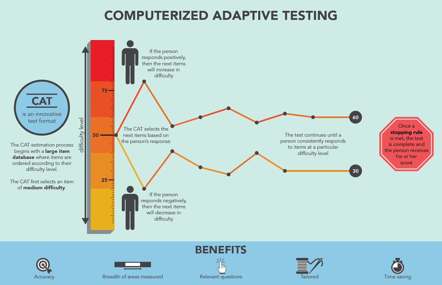
- Read the CAT Theory document to understand IRT concepts
Concerto Platform — Known Rules (From Experience)
Before building, understand these important rules discovered through testing:
| Rule | Detail |
|---|---|
| ✅ Use showPage not form | form node does not pass variables correctly |
| ✅ Enter HTML directly | Use the HTML field in showPage, not templates |
| ✅ Use Flow variable pointers | All data ports need ↑ (output) or ↓ (input) Flow variable pointer set |
| ✅ Use default out port | Do not use custom branch names or .branch |
| ✅ Use if node with variable | Pass a TRUE/FALSE variable to if node expression |
| ✅ Use SQL syntax | concerto.table.query("SELECT * FROM table") not table= argument |
| ❌ No custom .branch names | Custom execution ports with .branch don't work reliably |
| ❌ No form node | Variables don't pass through correctly |
| ❌ No table= argument | concerto.table.query(table="x") throws an error |
Concept: What is the 3PL Model (with Guessing)?
The 3-Parameter Logistic (3PL) model extends basic IRT by adding a guessing parameter (c) [2][5]:
Where:
- (theta) — test-taker's ability estimate (starts at 0)
- — discrimination: how well the item separates ability levels
- — difficulty: the ability level at which (ignoring guessing)
- — guessing: minimum probability of correct answer (e.g. 0.25 for 4-choice MCQ)
Why does guessing matter?
Without guessing (2PL), if theta is very low, . But in reality, a test-taker can still guess correctly — especially on multiple choice. The guessing parameter sets a floor on the probability [2]:
Item Information with Guessing
The information provided by a 3PL item is [3][5]:
Items with high discrimination () and difficulty near current theta () provide the most information [3][14].
Concept: Bayesian EAP Theta Estimation
This tutorial uses Bayesian Expected A Posteriori (EAP) estimation — the most robust method for CAT theta estimation [8][10].
Why Bayesian EAP instead of Newton-Raphson?
How EAP Works
EAP combines the likelihood of the observed responses with a prior distribution (our belief about ability before the test) [8]:
Where:
- — likelihood of all responses
- — standard normal prior (most people have average ability)
- — vector of responses (1=correct, 0=incorrect)
Numerical Approximation (used in our R code)
The integral is approximated using Gauss-Hermite quadrature — evaluating the integrand at a grid of theta points with weights [6][8]:
The Standard Error is also computed from the posterior variance:
Part 1: Create the Item Bank (Data Table)
Concept
The item bank stores all test questions along with their IRT parameters. The 3PL model requires three parameters per item: discrimination (), difficulty (), and guessing () [2][5][15].
Steps
- Click Data Tables in the left menu → Add new
- Name it item_bank_3pl
- Add these columns by clicking Add column:
| Column Name | Type | Description |
|---|---|---|
| question | string | The question text |
| option_a | string | Choice A |
| option_b | string | Choice B |
| option_c | string | Choice C |
| option_d | string | Choice D |
| correct_answer | string | Correct option: A, B, C, or D |
| difficulty | decimal | IRT parameter (range: -3 to +3) |
| discrimination | decimal | IRT parameter (range: 0 to 3) |
| guessing | decimal | IRT parameter (range: 0 to 0.35) |
- Click Save
- Click Edit data and add sample items with varying difficulty:
| question | option_a | option_b | option_c | option_d | correct_answer | difficulty | discrimination | guessing |
|---|---|---|---|---|---|---|---|---|
| What is 1+1? | 1 | 2 | 3 | 4 | B | -2.0 | 0.8 | 0.25 |
| What is 5-3? | 1 | 2 | 3 | 4 | B | -1.5 | 1.0 | 0.25 |
| What is 4x3? | 10 | 12 | 14 | 16 | B | -1.0 | 1.2 | 0.25 |
| What is 15/3? | 3 | 4 | 5 | 6 | C | -0.5 | 1.3 | 0.25 |
| What is 7x8? | 54 | 56 | 58 | 60 | B | 0.0 | 1.5 | 0.25 |
| What is 12²? | 124 | 140 | 144 | 148 | C | 0.5 | 1.4 | 0.25 |
| What is √169? | 11 | 12 | 13 | 14 | C | 1.0 | 1.6 | 0.25 |
| What is 17x13? | 201 | 211 | 221 | 231 | C | 1.5 | 1.7 | 0.25 |
| What is 2^10? | 512 | 1024 | 2048 | 4096 | B | 2.0 | 1.8 | 0.25 |
| What is log₂(256)? | 6 | 7 | 8 | 9 | C | 2.5 | 2.0 | 0.25 |
- Click Save
Note: All guessing values are 0.25 because these are 4-choice MCQ items. The probability of guessing correctly = 1/4 = 0.25.
Part 2: Create the Test
- Click Tests → Add new → name it cat_3pl_test → Save
- Click the Test flow tab
- You will see test start and test end on the canvas
Part 3: Build the Test Flow
Final Flow Overview
[test start]
     ↓
[eval - init]           Initialize all variables + response history
     ↓
[eval - select item] ←──────────────────────────┐
     ↓                                           │
[showPage - question]   Show item to user        │
     ↓                                           │
[eval - score]          Score + Bayesian EAP     │
     ↓                                           │
[if]                    Test complete?           │
  │ false ──────────────────────────────────────┘
  │ true
  ↓
[eval - compute result] Compute labels + SE
     ↓
[showPage - result]     Show final score + SE
     ↓
[test end]
Node 1: eval - init — Initialize Variables
Concept
This node sets all starting values before the test begins. For Bayesian EAP, we also initialize:
- responses — a vector tracking all responses (1=correct, 0=incorrect) across items
- items_a, items_b, items_c — vectors tracking IRT parameters of answered items
- se_theta — the standard error of the theta estimate
- theta = 0 — prior mean (start at average ability) [12]
The response history vectors are essential for EAP because it needs all previous responses and item parameters to compute the posterior, not just the most recent one [8].
Steps
- Right-click canvas → eval
- Rename it to eval - init
- Click the node → edit Code field → paste:
# ── Ability estimate ──────────────────────────────────────────────────────────
# Start at population mean θ = 0 (prior mean for Bayesian EAP)
theta    <- 0

# ── Standard error of theta estimate ─────────────────────────────────────────
# Starts high (very uncertain), decreases as more items are answered
se_theta <- 999

# ── Test control variables ────────────────────────────────────────────────────
answered  <- 0      # number of items answered so far
max_items <- 10     # fixed-length stopping rule

# ── Used item tracking ────────────────────────────────────────────────────────
# Prevents the same item from being shown twice
used_items <- c()

# ── Response history — required for Bayesian EAP ─────────────────────────────
# responses: 1 = correct, 0 = incorrect, one entry per answered item
responses <- c()

# IRT parameter history — one entry per answered item (same order as responses)
items_a   <- c()   # discrimination parameters of answered items
items_b   <- c()   # difficulty parameters of answered items
items_c   <- c()   # guessing parameters of answered items

# ── Question display variables ────────────────────────────────────────────────
correct_answer <- ""
question       <- ""
option_a       <- ""
option_b       <- ""
option_c       <- ""
option_d       <- ""
current_id     <- 0

# ── Scoring totals ────────────────────────────────────────────────────────────
total_correct <- 0
test_complete <- FALSE- Click Save
Add output ports (↑)
Click red + for each variable. Then click each port → check Flow variable pointer → set Pointed variable name to the same name → Save:
- theta
- se_theta
- answered
- max_items
- used_items
- responses
- items_a
- items_b
- items_c
- correct_answer
- question
- option_a
- option_b
- option_c
- option_d
- current_id
- total_correct
- test_complete
Each should show a ↑ arrow when done.
Connect
Drag from test start out → eval - init in
Details
The eval - init node runs exactly once — at the very beginning of the test, immediately after test start. Its sole purpose is to initialize every variable that will be used throughout the entire CAT session.
It is the simplest node in the flow but also the most foundational: if any variable is missing or wrongly typed here, every subsequent node will fail.
| Property | Value |
|---|---|
| Runs | Once only — at test start |
| Position in flow | test start → eval - init → eval - select item |
| Purpose | Initialize all session variables with correct types and starting values |
| Outputs | All variables needed by every other node |
Complete R Code
# ── Ability estimate ──────────────────────────────────────────────────────────
# Start at population mean θ = 0 (prior mean for Bayesian EAP)
theta    <- 0

# ── Standard error of theta estimate ─────────────────────────────────────────
# Starts high (very uncertain), decreases as more items are answered
se_theta <- 999

# ── Test control variables ────────────────────────────────────────────────────
answered  <- 0      # number of items answered so far
max_items <- 10     # fixed-length stopping rule

# ── Used item tracking ────────────────────────────────────────────────────────
# Prevents the same item from being shown twice
used_items <- numeric(0)

# ── Response history — required for Bayesian EAP ─────────────────────────────
# responses: 1 = correct, 0 = incorrect, one entry per answered item
responses <- numeric(0)

# IRT parameter history — one entry per answered item (same order as responses)
items_a   <- numeric(0)   # discrimination parameters of answered items
items_b   <- numeric(0)   # difficulty parameters of answered items
items_c   <- numeric(0)   # guessing parameters of answered items

# ── Question display variables ────────────────────────────────────────────────
correct_answer <- ""
question       <- ""
option_a       <- ""
option_b       <- ""
option_c       <- ""
option_d       <- ""
current_id     <- 0

# ── Scoring totals ────────────────────────────────────────────────────────────
total_correct <- 0
test_complete <- FALSE
Variable-by-Variable Explanation
theta <- 0
What it is: The current ability estimate — the CAT's best guess of the test-taker's true latent ability on the IRT scale.
theta <- 0Why start at 0: In IRT, the ability scale is standardized so that the population mean is 0 and the standard deviation is 1. Starting at means we begin with the assumption that the test-taker has average ability — the most neutral and statistically justified starting point before any evidence is collected.
This is the prior mean of the Bayesian EAP estimation. The standard normal prior used in eval - score is centered at 0, so starting theta at 0 is consistent with the prior.
What happens if we started elsewhere:
| Starting theta | Effect |
|---|---|
| Neutral — most appropriate for unknown test-takers | |
| First item will be easier than necessary — wastes 1 item | |
| First item will be too hard — may discourage test-taker | |
| Efficient if we have prior information (e.g., previous test) |
How theta evolves:
Start:    theta = 0.0000  (prior mean, no data)
After Q1: theta = 0.3821  (answered correctly — ability estimate rises)
After Q2: theta = 0.1504  (answered incorrectly — estimate falls)
After Q3: theta = 0.2813  (answered correctly — rises again)
...
After Q10: theta = 0.4217  (converged estimate)
The EAP algorithm in eval - score updates this value after every response.
se_theta <- 999
What it is: The Standard Error of the theta estimate — a measure of how precisely we know the test-taker's ability:
se_theta <- 999Why 999 and not 0, NA, or Inf:
Before any items are answered (), the true SE is mathematically infinite:
We cannot use Inf directly because Concerto may corrupt infinite values during flow variable serialization. 999 is a sentinel value — a deliberately large finite number that means "infinitely uncertain":
| Value | Problem |
|---|---|
| Inf | May not serialize correctly through Concerto flow pointers |
| NA | Causes arithmetic errors in CI calculation: 0 ± 1.96 * NA → NA |
| 0 | Implies perfect precision — dangerously wrong |
| 999 | ✅ Safely serializable, obviously not a real SE, makes all stopping rules evaluate correctly |
Why it matters for the stopping rule: In eval - score, the SE-based stopping rule is:
test_complete <- (se_theta < 0.3) | (answered >= max_items)With se_theta = 999 initially:
999 < 0.3 # → FALSE ✅ test correctly does not stop before any itemsIf se_theta were 0:
0 < 0.3 # → TRUE ❌ test would immediately end with zero items answeredHow SE evolves:
| After item | Typical SE | Interpretation |
|---|---|---|
| 0 (init) | 999 | Sentinel — no data |
| 1 | ~0.89 | Very uncertain |
| 3 | ~0.62 | Improving |
| 5 | ~0.48 | Acceptable |
| 7 | ~0.38 | Good |
| 10 | ~0.31 | High precision |
SE is a real EAP-computed value from item 1 onward — 999 exists only for the single moment before the first item is shown.
answered <- 0
What it is: A counter tracking how many items have been answered so far.
answered <- 0Why start at 0: No items have been answered at test start. This counter increments by 1 in eval - score after each submission:
# In eval - score:
answered <- as.numeric(answered) + 1
How it is used:
| Node | Use of answered |
|---|---|
| showPage - question | Displays "Question {{answered}} of {{max_items}}" |
| eval - score | Incremented after each response |
| eval - score | Used in stopping rule: n_answered >= max_items |
| showPage - result | Shows total items answered |
| eval - compute result | Used for percentage correct calculation |
Why integer not logical: answered participates in arithmetic (answered + 1) and comparison (answered >= max_items), so it must be numeric. Starting as 0 (integer) ensures this.
max_items <- 10
What it is: The fixed-length stopping rule threshold — the maximum number of items the test will administer.
max_items <- 10Why 10: 10 is a reasonable default for a demonstration CAT. In operational CATs:
| Test type | Typical length |
|---|---|
| Demonstration / prototype | 5–10 items |
| Short-form CAT | 10–20 items |
| Standard CAT | 20–40 items |
| High-stakes certification (e.g. NCLEX) | 75–145 items |
To change the test length: Simply change this one value:
max_items <- 5    # short demo
max_items <- 20   # standard test
max_items <- 30   # longer assessment
How it flows through the system:
eval - init:     max_items = 10  (set here)
      ↓ output ↑
eval - select item: receives max_items, passes to showPage
      ↓
showPage - question: displays "Question X of 10"
      ↓
eval - score:    max_items received, used in:
                 test_complete <- n_answered >= max_items
Why defined here and not hardcoded in eval - score: Centralizing configuration in eval - init means you only need to change one place to adjust test length. If it were hardcoded in eval - score, you would need to update two nodes whenever you changed the test length.
used_items <- numeric(0)
What it is: A vector tracking the IDs of all items that have already been administered. Used in eval - select item to exclude already-seen items from selection.
used_items <- numeric(0)Why numeric(0) and not c() or NULL:
| Initialization | Type | Problem |
|---|---|---|
| c() | NULL | length(NULL) = 0 works, but type is ambiguous |
| NULL | NULL | c(NULL, 5) → 5 but Concerto may serialize NULL differently |
| numeric(0) | numeric | ✅ Explicitly numeric, empty vector of correct type |
Using numeric(0) ensures that when we later do c(used_items, current_id) where current_id is an integer, the result is always a numeric vector — never a character or list.
How it is used in eval - select item:
if (length(used_items) > 0) {
  items <- items[!items$id %in% used_items, ]
}
On the first call: length(numeric(0)) = 0 → condition is FALSE → filter skipped → all items available.
Progression across the test:
# Before Q1:  numeric(0)         → all 10 items available
# Before Q2:  c(5)               → 9 items available
# Before Q3:  c(5, 6)            → 8 items available
# Before Q10: c(5,6,3,7,1,9,4,8,10) → 1 item remaining
responses <- numeric(0)
What it is: A vector storing the binary response history — one entry per answered item:
- 1 = correct
- 0 = incorrect
responses <- numeric(0)This is the vector in the EAP likelihood formula:
Why this is critical for Bayesian EAP: Unlike Newton-Raphson (which uses only the most recent item), EAP recomputes theta from scratch after every item using all previous responses. Without this vector, EAP cannot function — it needs the complete response history to compute the likelihood.
Why numeric(0) not c(): Same reasoning as used_items — explicit numeric type prevents type errors when arithmetic is performed on elements in the EAP loop.
Progression across the test:
# Before Q1:  numeric(0)      → no responses yet
# After Q1:   c(0)            → answered incorrectly
# After Q2:   c(0, 1)         → Q2 correct
# After Q3:   c(0, 1, 1)      → Q3 correct
# After Q10:  c(0,1,1,0,1,0,1,1,0,1) → full history
In eval - score, the new response is appended:
responses <- c(responses, is_correct)items_a <- numeric(0), items_b <- numeric(0), items_c <- numeric(0)
What they are: Three parallel vectors that store the IRT parameters of every item that has been answered, in the same order as responses.
items_a <- numeric(0)   # discrimination parameters of answered items
items_b <- numeric(0)   # difficulty parameters of answered items
items_c <- numeric(0)   # guessing parameters of answered items
Why three separate vectors: The EAP inner loop in eval - score iterates over answered items and needs all three parameters for each:
for (j in seq_len(n_answered)) {
  Pj <- items_c[j] + (1 - items_c[j]) / (1 + exp(-items_a[j] * (th - items_b[j])))
  ...
}
Storing them as separate parallel numeric vectors (rather than a data frame or list) makes element-wise access inside the loop reliable and avoids type coercion issues.
Why numeric(0) not c(): The EAP code does arithmetic on these vectors (1 - items_c[j], -items_a[j] * ...). Initializing as numeric(0) guarantees they are numeric before any elements are appended.
Parallel structure — they must always have the same length:
# After 3 items (responses = c(0, 1, 1)):
items_a <- c(0.8, 1.5, 1.4)    # item 1: a=0.8, item 2: a=1.5, item 3: a=1.4
items_b <- c(-2.0, 0.0, 0.5)   # item 1: b=-2.0, etc.
items_c <- c(0.25, 0.25, 0.25)  # all 4-choice MCQ so c=0.25 for all

# Invariant: length(responses) == length(items_a) == length(items_b) == length(items_c)
In eval - score, all four vectors are appended together in the same block:
responses <- c(responses, is_correct)
items_a   <- c(items_a,   a_new)
items_b   <- c(items_b,   b_new)
items_c   <- c(items_c,   c_new)
This guarantees the parallel structure is maintained across all iterations.
Question Display Variables
What they are: Placeholder variables for the current item's content. These are populated by eval - select item before each question is shown.
correct_answer <- ""
question       <- ""
option_a       <- ""
option_b       <- ""
option_c       <- ""
option_d       <- ""
current_id     <- 0
Why initialize as empty strings: These variables must exist as flow variables from the very first node. If they were not initialized here, eval - select item might receive NULL on the first iteration, causing errors during type conversion or string operations.
Why current_id <- 0 (not numeric(0)): current_id is used in a SQL WHERE clause in eval - score:
paste0("SELECT * FROM item_bank_3pl WHERE id = ", current_id)An ID of 0 produces valid (if harmless) SQL: WHERE id = 0. This will return zero rows — safely handled. By contrast, numeric(0) would produce WHERE id = (incomplete SQL — an error).
Flow of display variables:
eval - init:          question = ""    (blank placeholder)
      ↓
eval - select item:   question = "What is 7x8?"   (filled by item selection)
      ↓
showPage - question:  {{question}} → "What is 7x8?"   (displayed to user)
      ↓
eval - score:         correct_answer used for scoring
      ↓
eval - select item:   question = "What is √169?"  (next item, overwrites)
      ↓
showPage - question:  {{question}} → "What is √169?"
total_correct <- 0
What it is: A running count of how many items the test-taker answered correctly.
total_correct <- 0How it is updated in eval - score:
is_correct    <- as.integer(answer == correct_answer)
total_correct <- as.numeric(total_correct) + is_correct
How it is used in eval - compute result:
pct_correct <- round((total_correct / answered) * 100, 1)Why this is separate from theta: total_correct is a classical test theory metric (raw score / percentage correct). Theta is an IRT metric. They measure the same construct differently:
| Metric | Type | Range | Properties |
|---|---|---|---|
| total_correct | Classical | 0 to max_items | Simple count, scale-dependent |
| theta | IRT | to | Scale-independent, comparable across test forms |
Both are reported on the results page to give test-takers a familiar score alongside the IRT estimate.
test_complete <- FALSE
What it is: A logical flag that controls whether the if node routes to the next item or to the results page.
test_complete <- FALSEWhy initialize as FALSE: At test start, the test is obviously not complete. Initializing as FALSE means the if node expression test_complete evaluates correctly on the first pass without errors.
How it is updated in eval - score:
test_complete <- n_answered >= max_itemsHow the if node uses it:
test_complete = FALSE  →  if node "false" port  →  loop back to eval - select item
test_complete = TRUE   →  if node "true" port   →  go to eval - compute result
Why logical not integer: The if node expression field expects a logical (TRUE/FALSE) value. If test_complete were an integer (0 or 1), the if node might not evaluate it correctly. Initializing as FALSE (logical) and keeping it as logical throughout avoids this issue.
Why Every Variable Must Be Initialized Here
Concerto flow variable pointers only work for variables that already exist in the R session. If a variable is first created in eval - select item or eval - score (instead of eval - init), it will not be available as a flow variable in earlier rounds when the loop returns to that node.
The pattern is:
eval - init creates ALL variables with correct types
      ↓
eval - select item reads some, overwrites some, passes all forward
      ↓
showPage - question reads some, adds `answer`
      ↓
eval - score reads all, updates some, passes all forward
      ↓
if node routes based on test_complete
      ↓
loop back to eval - select item (which now has updated values from eval - score)
If any variable is missing from eval - init, the first time the loop returns to eval - select item, that variable will be NULL — causing either a silent error or a crash.
Type Choices — Why They Matter
| Variable | Type | Why this type |
|---|---|---|
| theta | numeric (double) | IRT computations require decimal precision |
| se_theta | numeric (double) | SE is always a decimal; 999 is sentinel for ∞ |
| answered | numeric (integer-like) | Counter — arithmetic +1 must work |
| max_items | numeric (integer-like) | Comparison >= max_items must work |
| used_items | numeric(0) (empty numeric) | %in% comparison with integer IDs |
| responses | numeric(0) (empty numeric) | Arithmetic in EAP loop: u_j * log(P_j) |
| items_a/b/c | numeric(0) (empty numeric) | Arithmetic in EAP: exp(-a*(th-b)) |
| question etc | "" (character) | Template substitution requires strings |
| current_id | 0 (numeric) | SQL WHERE clause concatenation |
| total_correct | 0 (numeric) | Arithmetic += is_correct |
| test_complete | FALSE (logical) | if node expression evaluates logicals |
Summary
eval - init is the configuration and initialization hub of the entire CAT session. Its design principles are:
- Initialize everything — every variable used anywhere in the flow must be created here with the correct type
- Use safe types — numeric(0) for empty vectors, FALSE for logicals, 0 for numeric counters
- Use sentinel values — se_theta = 999 for "not yet computed" infinity
- Centralize configuration — max_items = 10 here means one place to change test length
- Export everything — every variable needs an output port with Flow variable pointer (↑)
Node 2: eval - select item — CAT Item Selection (3PL Maximum Information)
Concept
Selects the next item using the Maximum Information criterion based on the 3PL model [3][11][14].
Step 1: Compute for each remaining item [2]:
Step 2: Compute for each item [3][5]:
Steps
- Right-click canvas → eval
- Rename it to eval - select item
- Click the node → edit Code field → paste:
# ── Load all items from the item bank ─────────────────────────────────────────
items <- concerto.table.query("SELECT * FROM item_bank_3pl")

# ── Remove already-used items to prevent repetition ───────────────────────────
if (length(used_items) > 0) {
  items <- items[!items$id %in% used_items, ]
}

# ── Convert IRT parameter columns to numeric ───────────────────────────────────
items$difficulty     <- as.numeric(items$difficulty)
items$discrimination <- as.numeric(items$discrimination)
items$guessing       <- as.numeric(items$guessing)

# ── Extract IRT parameter vectors ─────────────────────────────────────────────
a <- items$discrimination
b <- items$difficulty
c <- items$guessing

# ── Step 1: Calculate P(θ) for each item using 3PL formula ───────────────────
# P(θ) = c + (1-c) / (1 + exp(-a*(θ-b)))
P <- c + (1 - c) / (1 + exp(-a * (theta - b)))

# ── Step 2: Calculate Item Information I(θ) ───────────────────────────────────
# I(θ) = a² * [(P-c)²/(1-c)²] * [(1-P)/P]
# Safety: prevent division by zero when P ≈ 0 or P ≈ 1
P_safe <- pmax(pmin(P, 0.9999), 0.0001)
items$information <- (a^2) * ((P_safe - c)^2 / (1 - c)^2) * ((1 - P_safe) / P_safe)

# ── Step 3: Select item with maximum information ───────────────────────────────
selected <- items[which.max(items$information), ]

# ── Set question display variables ────────────────────────────────────────────
question       <- as.character(selected$question)
option_a       <- as.character(selected$option_a)
option_b       <- as.character(selected$option_b)
option_c       <- as.character(selected$option_c)
option_d       <- as.character(selected$option_d)
correct_answer <- as.character(selected$correct_answer)
current_id     <- as.integer(selected$id)

# ── Track this item as used ───────────────────────────────────────────────────
used_items <- c(used_items, current_id)- Click Save
Add input ports (↓)
Click blue + for each. Click each port → check Flow variable pointer → Pointed variable name → Save:
- theta
- answered
- max_items
- used_items
Add output ports (↑)
Click red + for each. Click each port → check Flow variable pointer → Pointed variable name → Save:
- question
- option_a
- option_b
- option_c
- option_d
- correct_answer
- current_id
- used_items
- answered
- max_items
- theta
Connect
Drag from eval - init out → eval - select item in
Details
The eval - select item node runs at the start of every CAT loop iteration — once before each question is shown. It is the implementation of the CAT item selection algorithm: given the current ability estimate , it selects the most informative unused item from the bank.
It performs four sequential tasks:
| Task | Description |
|---|---|
| Task 1 | Load all items from the database |
| Task 2 | Filter out already-used items |
| Task 3 | Compute 3PL information for each remaining item |
| Task 4 | Select the item with maximum information and set display variables |
Task 1: Load All Items from the Database
items <- concerto.table.query("SELECT * FROM item_bank_3pl")What it does
Queries the entire item_bank_3pl table and returns all rows as an R data frame stored in items.
Why SELECT *
We need all columns — question text, options, correct answer, and IRT parameters — so SELECT * retrieves everything in one call. A more targeted query like SELECT id, discrimination, difficulty, guessing would be faster for large banks, but for typical CAT banks of 50–200 items the difference is negligible.
What items looks like after this line
| id | question | option_a | option_b | option_c | option_d | correct_answer | difficulty | discrimination | guessing |
|---|---|---|---|---|---|---|---|---|---|
| 1 | What is 1+1? | 1 | 2 | 3 | 4 | B | -2.0 | 0.8 | 0.25 |
| 2 | What is 5-3? | 1 | 2 | 3 | 4 | B | -1.5 | 1.0 | 0.25 |
| 3 | What is 4x3? | 10 | 12 | 14 | 16 | B | -1.0 | 1.2 | 0.25 |
| ... | ... | ... | ... | ... | ... | ... | ... | ... | ... |
| 10 | What is log₂(256)? | 6 | 7 | 8 | 9 | C | 2.5 | 2.0 | 0.25 |
Data types from Concerto database
Concerto returns all database values as character strings by default, regardless of the column type declared in the Data Table. This is why explicit type conversion is always required before any mathematical operations.
Task 2: Filter Out Already-Used Items
if (length(used_items) > 0) {
  items <- items[!items$id %in% used_items, ]
}
Mathematical notation
This implements the constraint in the item selection rule:
Where is the set of already-used item IDs.
Line-by-line breakdown
length(used_items) > 0
Checks whether any items have already been administered. On the very first question, used_items was initialized as numeric(0) (an empty vector) in eval - init, so length(numeric(0)) = 0 and the filter block is skipped entirely — all items remain available.
From question 2 onward, used_items grows by one ID per answered item, so the filter runs.
# Before question 1:
used_items <- numeric(0)
length(used_items)        # → 0  → skip filter

# Before question 2 (item 5 was used):
used_items <- c(5)
length(used_items)        # → 1  → run filter
items$id %in% used_items
The %in% operator checks membership. For each element of items$id, returns TRUE if that ID is in used_items, FALSE otherwise:
items$id    <- c(1, 2, 3, 4, 5, 6, 7, 8, 9, 10)
used_items  <- c(5, 3, 7)

items$id %in% used_items
# → c(FALSE, FALSE, TRUE, FALSE, TRUE, FALSE, TRUE, FALSE, FALSE, FALSE)
#          1      2     3      4     5      6     7      8      9     10
Items 3, 5, and 7 were already used → TRUE.
!items$id %in% used_items
The ! operator flips all logical values — keeping items that are not in used_items:
!c(FALSE, FALSE, TRUE, FALSE, TRUE, FALSE, TRUE, FALSE, FALSE, FALSE)
# →  c(TRUE,  TRUE, FALSE, TRUE, FALSE,  TRUE, FALSE,  TRUE,  TRUE,  TRUE)
Items 1, 2, 4, 6, 8, 9, 10 remain → these are the candidates for selection.
items[..., ]
Subsets the data frame — keeping only rows where the logical vector is TRUE:
items <- items[c(TRUE, TRUE, FALSE, TRUE, FALSE, TRUE, FALSE, TRUE, TRUE, TRUE), ]
# Keeps rows for items 1, 2, 4, 6, 8, 9, 10
# Removes rows for items 3, 5, 7 (already used)
The trailing comma in items[condition, ] is required in R to indicate we are subsetting rows (not columns).
Progression across the test
| Before question | used_items | Items remaining |
|---|---|---|
| Q1 | numeric(0) | 10 of 10 |
| Q2 | c(5) | 9 of 10 |
| Q3 | c(5, 3) | 8 of 10 |
| Q4 | c(5, 3, 7) | 7 of 10 |
| Q10 | c(5,3,7,1,9,2,6,8,4) | 1 of 10 |
Task 3: Type Conversion and Parameter Extraction
Convert IRT columns to numeric
items$difficulty     <- as.numeric(items$difficulty)
items$discrimination <- as.numeric(items$discrimination)
items$guessing       <- as.numeric(items$guessing)
As noted above, Concerto returns all database values as character strings. Without this conversion:
# What Concerto returns:
items$difficulty[1]      # → "0.5"   (a string)

# What happens without conversion:
0.5 - "0.5"              # → Error: non-numeric argument to binary operator

# What happens with conversion:
as.numeric("0.5") - 0.5  # → 0.0   ✅
Only the three IRT parameter columns need conversion here. The question text and options remain as character strings (which is correct for display).
Extract parameter vectors
a <- items$discrimination
b <- items$difficulty
c <- items$guessing
Pulls the three IRT parameter columns into standalone vectors a, b, c.
Why create separate vectors?
R is vectorized — arithmetic operations on vectors are applied element-wise across all elements simultaneously, without explicit loops:
a <- c(0.8, 1.0, 1.2, 1.5, 1.8)   # 5 items
b <- c(-2.0, -1.0, 0.0, 1.0, 2.0)
c <- c(0.25, 0.25, 0.25, 0.25, 0.25)
theta <- 0.0

# This computes P for ALL 5 items at once:
P <- c + (1 - c) / (1 + exp(-a * (theta - b)))
# → c(0.969, 0.938, 0.625, 0.312, 0.254)
This is equivalent to running a for-loop over all items but is:
- Faster — implemented in compiled C internally
- Cleaner — no loop boilerplate
- Less error-prone — no index management
Task 4: Calculate P(θ) for All Items
P <- c + (1 - c) / (1 + exp(-a * (theta - b)))The 3PL Model
This implements the 3-Parameter Logistic (3PL) Item Characteristic Curve:
Where:
- — current ability estimate (scalar, same for all items)
- — discrimination parameter of item
- — difficulty parameter of item
- — guessing parameter of item
Breaking down the formula component by component
| Component | Code | Mathematical role |
|---|---|---|
| theta - b | Distance between ability and difficulty | |
| -a * (theta - b) | Scaled, negated distance | |
| exp(-a * (theta - b)) | Exponential — always positive | |
| 1 / (1 + exp(...)) | Logistic function — maps | |
| (1-c) / (1+exp(...)) | Scaled by to fit in | |
| c + ... | Shifts up by — sets the lower asymptote |
Role of each parameter
Difficulty — where on the theta scale P = 0.5 + c/2
The difficulty parameter shifts the curve left or right along the theta axis. At (ignoring guessing, ):
With guessing (), the inflection point is slightly above .
Low b (easy item):          High b (hard item):
P                           P
1.0 ──────────              1.0         ──────────
0.5 ──┐                     0.5               ──┐
0.25  │ (guessing)          0.25 (guessing)   │
      └────                             └────
      θ                                       θ
   b=-2.0                               b=+2.0
Discrimination — steepness of the curve
Higher means the curve rises more steeply — the item more sharply separates test-takers above vs below the difficulty level:
High a (steep):     Low a (shallow):
P                   P
1.0  ─┐             1.0    ──────────
0.5  ─┤             0.5   ─
0.25  │             0.25 ─
     ─┘
      θ=b            θ=b
Guessing — lower asymptote
Sets the floor on . Even at , :
For 4-choice MCQ items: (random guessing = 1/4).
Concrete example at
For 10 items with increasing difficulty ( from -2.0 to +2.5):
| Item | ||||||
|---|---|---|---|---|---|---|
| 1 | 0.8 | -2.0 | 0.25 | 2.0 | 0.969 | |
| 2 | 1.0 | -1.5 | 0.25 | 1.5 | 0.938 | |
| 3 | 1.2 | -1.0 | 0.25 | 1.0 | 0.886 | |
| 4 | 1.3 | -0.5 | 0.25 | 0.5 | 0.794 | |
| 5 | 1.5 | 0.0 | 0.25 | 0.0 | 0.625 | |
| 6 | 1.4 | 0.5 | 0.25 | -0.5 | 0.431 | |
| 7 | 1.6 | 1.0 | 0.25 | -1.0 | 0.305 | |
| 8 | 1.7 | 1.5 | 0.25 | -1.5 | 0.266 | |
| 9 | 1.8 | 2.0 | 0.25 | -2.0 | 0.254 | |
| 10 | 2.0 | 2.5 | 0.25 | -2.5 | 0.250 |
At , easy items have high (near 1), hard items approach the guessing floor (0.25).
Task 5: Calculate Item Information I(θ)
P_safe <- pmax(pmin(P, 0.9999), 0.0001)
items$information <- (a^2) * ((P_safe - c)^2 / (1 - c)^2) * ((1 - P_safe) / P_safe)
The 3PL Item Information Function (IIF)
The Item Information Function measures how much statistical information item provides about at a given ability level:
Why two lines? — Probability clamping
P_safe <- pmax(pmin(P, 0.9999), 0.0001)The IIF formula has in the denominator — division by becomes a problem when , and . Similarly, the term is invalid if due to floating point errors.
pmin(P, 0.9999) — element-wise minimum: caps each at 0.9999:
pmin(c(0.9999, 1.0000, 0.8), 0.9999)
# → c(0.9999, 0.9999, 0.8)
pmax(..., 0.0001) — element-wise maximum: floors each result at 0.0001:
pmax(c(0.0001, 0.0000, 0.5), 0.0001)
# → c(0.0001, 0.0001, 0.5)
Note: pmax/pmin (lowercase p) operate element-wise on vectors, unlike max/min which return a single scalar. This is important here since P is a vector of 10 values.
Breaking down the IIF formula
Component 1: — Discrimination squared
Items with higher discrimination contribute quadratically more information. An item with provides more information (at its peak) than one with .
a^2| Relative contribution | ||
|---|---|---|
| 0.5 | 0.25 | Low |
| 1.0 | 1.00 | Baseline |
| 1.5 | 2.25 | 2.25× |
| 2.0 | 4.00 | 4× |
Component 2: — Guessing correction
This term scales down the information to account for the guessing floor. It equals , which is the proportion of the probability above the guessing floor relative to the maximum possible.
(P_safe - c)^2 / (1 - c)^2At the difficulty point (, where ):
So the guessing parameter reduces peak information by factor . For : reduction factor = — guessing cuts peak information nearly in half.
Component 3: — Uncertainty term
This term is maximized when and approaches 0 at both extremes:
| Interpretation | ||
|---|---|---|
| 0.25 (guessing floor) | 3.00 | All uncertainty is guessing — not true ability |
| 0.5 | 1.00 | Maximum genuine uncertainty |
| 0.75 | 0.33 | Mostly correct — less to learn |
| 0.99 | 0.01 | Near-certain — item too easy |
| 0.01 | 99.0 | But clamped — item too hard |
(1 - P_safe) / P_safeCombined with the guessing correction, the true maximum information for a 3PL item occurs slightly above the difficulty parameter , not exactly at it, because the guessing floor shifts the optimal point upward.
Where is information maximized?
Information is maximized where — items work best when difficulty matches ability:
I(θ)
  │         ╭─────╮         ← Item with b=0.5 (peaks near θ=0.5)
  │        ╭╯     ╰╮
  │      ╭─╯       ╰─╮
  │   ╭──╯           ╰──╮
  │╭──╯                 ╰──╮
  └────────────────────────── θ
  -3  -2  -1   0   1   2   3
                  ↑
b = 0.5- Items too easy (): , uncertainty term , information drops
- Items too hard (): , guessing correction , information drops
- Items well-matched (): both terms are at reasonable values, information peaks
Concrete example at
Using values from the table above:
| Item | ||||||||
|---|---|---|---|---|---|---|---|---|
| 1 | 0.8 | -2.0 | 0.25 | 0.969 | 0.64 | 0.656 | 0.032 | 0.013 |
| 2 | 1.0 | -1.5 | 0.25 | 0.938 | 1.00 | 0.564 | 0.066 | 0.037 |
| 3 | 1.2 | -1.0 | 0.25 | 0.886 | 1.44 | 0.430 | 0.129 | 0.080 |
| 4 | 1.3 | -0.5 | 0.25 | 0.794 | 1.69 | 0.295 | 0.259 | 0.129 |
| 5 | 1.5 | 0.0 | 0.25 | 0.625 | 2.25 | 0.250 | 0.600 | 0.338 |
| 6 | 1.4 | 0.5 | 0.25 | 0.431 | 1.96 | 0.082 | 1.320 | 0.212 |
| 7 | 1.6 | 1.0 | 0.25 | 0.305 | 2.56 | 0.014 | 2.279 | 0.082 |
| 8 | 1.7 | 1.5 | 0.25 | 0.266 | 2.89 | 0.002 | 2.759 | 0.016 |
| 9 | 1.8 | 2.0 | 0.25 | 0.254 | 3.24 | 0.0002 | 2.937 | 0.002 |
| 10 | 2.0 | 2.5 | 0.25 | 0.250 | 4.00 | ~0 | 3.000 | ~0 |
Item 5 (difficulty = 0.0, closest to ) has the highest information at 0.338. This will be selected.
Task 6: Select Maximum Information Item
selected <- items[which.max(items$information), ]which.max()
Returns the row index of the maximum value in a vector:
items$information <- c(0.013, 0.037, 0.080, 0.129, 0.338, 0.212, 0.082, 0.016, 0.002, 0.000)
which.max(items$information)   # → 5  (index of item 5)
This implements the Maximum Information selection criterion:
items[5, ]
Selects the entire row for item 5 — all columns (question, options, parameters):
selected <- items[5, ]
# A data frame with 1 row, all columns
The trailing comma is essential: items[5, ] selects row 5 (all columns). Without it, items[5] would select column 5 instead.
Task 7: Set Display Variables
question       <- as.character(selected$question)
option_a       <- as.character(selected$option_a)
option_b       <- as.character(selected$option_b)
option_c       <- as.character(selected$option_c)
option_d       <- as.character(selected$option_d)
correct_answer <- as.character(selected$correct_answer)
current_id     <- as.integer(selected$id)
Why as.character()?
When a column is extracted from a data frame row, R may return a factor level instead of a plain string, especially for character columns. Factor levels do not always behave like strings in template substitution:
# Without conversion:
selected$question   # → factor with level "What is 7x8?"
# Template: {{question}} might fail or show the factor level number

# With conversion:
as.character(selected$question)   # → "What is 7x8?"   plain string ✅
Why as.integer() for current_id?
current_id is used later in eval - score inside a SQL WHERE clause:
paste0("SELECT * FROM item_bank_3pl WHERE id = ", current_id)If current_id is a string "5", this produces valid SQL: WHERE id = 5. But making it an integer explicitly ensures correct behavior and prevents potential quoting issues in edge cases:
as.integer("5") # → 5L (integer)These variables are passed to showPage - question via flow pointers
The {{variable}} placeholders in the HTML template are replaced by these variable values:
<div class="question">{{question}}</div>
<!-- becomes: -->
<div class="question">What is 7x8?</div>
Task 8: Track the Used Item
used_items <- c(used_items, current_id)What it does
Appends current_id to the used_items vector, recording that this item has been administered.
Why this must happen in eval - select item not eval - score
The item ID must be tracked before the item is shown, not after it is scored. If the test-taker closes the browser mid-question (after seeing but before submitting), the eval - score node never runs. Tracking in eval - select item ensures the item is always recorded as used even in this edge case.
Progression across the test
# Before Q1: used_items = numeric(0)
# After Q1 selection (item 5):  used_items = c(5)
# After Q2 selection (item 6):  used_items = c(5, 6)
# After Q3 selection (item 3):  used_items = c(5, 6, 3)
# ...
# After Q10 selection (item 2): used_items = c(5, 6, 3, 7, 1, 9, 4, 8, 10, 2)
This vector is passed back via output flow variable pointer (↑) so the next iteration of eval - select item can filter it out.
How Item Selection Adapts Across the Test
The key insight is that theta changes after every item (updated by eval - score), and eval - select item always uses the latest theta. This creates the adaptive cycle:
Round 1: theta = 0.0  → select item with b closest to 0.0 → item 5 (b=0.0)
         Test-taker answers CORRECTLY
         EAP update: theta = 0.38

Round 2: theta = 0.38 → select item with max I(0.38) from remaining 9 items
         → item 6 (b=0.5) now optimal (closest to 0.38)
         Test-taker answers INCORRECTLY
         EAP update: theta = 0.15

Round 3: theta = 0.15 → select item with max I(0.15) from remaining 8 items
         → item 6 already used, next best is item 4 (b=-0.5) or item 5 (b=0.0)
         ...
The test converges on the true ability through this iterative approximation process.
Why Maximum Information is the Right Criterion
Fisher Information and theta estimation
The Fisher Information is the expected value of the squared score function:
For IRT, this simplifies to the Item Information Function . The Cramér-Rao lower bound states that no unbiased estimator can have variance smaller than:
Therefore, maximizing the total information minimizes the estimation variance. By selecting the item with the highest at each step, CAT greedily minimizes the variance of the final theta estimate with each question.
Comparison with simpler alternatives
| Method | Formula | Advantage | Disadvantage |
|---|---|---|---|
| Maximum Information (used here) | Optimal for precision | Can overexpose certain items | |
| b-matching | Simple, fast | Ignores discrimination | |
| Random | uniform random from pool | Maximum exposure control | No precision optimization |
| Randomesque | random among top-5 by | Balance of both | Slightly suboptimal |
For our 10-item demonstration CAT, Maximum Information is appropriate. For operational CATs with security requirements, exposure control methods (Sympson-Hetter, randomesque) are preferred.
Node 3: showPage - question — Display Question
Concept
Presents the selected item to the test-taker. We use showPage (not form) because it reliably receives flow variables via Flow variable pointers.
Steps
- Right-click canvas → showPage
- Rename it to showPage - question
- Click the node → find HTML field → click edit icon → paste:
<!DOCTYPE html>
<html>
<head>
  <style>
    * { box-sizing: border-box; margin: 0; padding: 0; }
    body {
      font-family: Arial, sans-serif;
      background: #f5f5f5;
      display: flex;
      justify-content: center;
      align-items: flex-start;
      min-height: 100vh;
      padding: 40px 20px;
    }
    .card {
      background: white;
      border-radius: 8px;
      box-shadow: 0 2px 8px rgba(0,0,0,0.1);
      padding: 32px;
      max-width: 640px;
      width: 100%;
    }
    .progress {
      font-size: 13px;
      color: #888;
      margin-bottom: 8px;
    }
    .progress-bar-bg {
      background: #e0e0e0;
      border-radius: 4px;
      height: 6px;
      margin-bottom: 24px;
    }
    .progress-bar-fill {
      background: #4a90e2;
      border-radius: 4px;
      height: 6px;
      width: calc({{answered}} / {{max_items}} * 100%);
    }
    .question {
      font-size: 18px;
      font-weight: bold;
      color: #333;
      margin-bottom: 24px;
      line-height: 1.5;
    }
    .options label {
      display: flex;
      align-items: center;
      padding: 12px 16px;
      border: 2px solid #e0e0e0;
      border-radius: 6px;
      margin-bottom: 10px;
      cursor: pointer;
      font-size: 15px;
      color: #444;
      transition: border-color 0.2s;
    }
    .options label:hover { border-color: #4a90e2; }
    .options input[type="radio"] { margin-right: 12px; }
    .btn-next {
      margin-top: 24px;
      width: 100%;
      padding: 14px;
      background: #4a90e2;
      color: white;
      font-size: 16px;
      border: none;
      border-radius: 6px;
      cursor: pointer;
    }
    .btn-next:hover { background: #357abd; }
  </style>
</head>
<body>
  <div class="card">
    <div class="progress">Question {{answered}} of {{max_items}}</div>
    <div class="progress-bar-bg">
      <div class="progress-bar-fill"></div>
    </div>
    <div class="question">{{question}}</div>
    <div class="options">
      <label><input type="radio" name="answer" value="A"> {{option_a}}</label>
      <label><input type="radio" name="answer" value="B"> {{option_b}}</label>
      <label><input type="radio" name="answer" value="C"> {{option_c}}</label>
      <label><input type="radio" name="answer" value="D"> {{option_d}}</label>
    </div>
    <button class="btn-next" type="submit">Next →</button>
  </div>
</body>
</html>- Click Save
Add input ports (↓)
Click blue + for each. Click each port → check Flow variable pointer → Pointed variable name → Save:
- question
- option_a
- option_b
- option_c
- option_d
- answered
- max_items
Add output port (↑)
Click red + → name it answer → click it → check Flow variable pointer → Pointed variable name: answer → Save
Connect
Drag from eval - select item out → showPage - question in
Node 4: eval - score — Score Response + Bayesian EAP Theta Estimation
Concept
This is the most important node. It performs three tasks after each response:
Task 1 — Score the response
Compare the submitted answer to correct_answer:
Task 2 — Update theta using Bayesian EAP
EAP treats theta estimation as a Bayesian inference problem [8]. After collecting responses :
(a) Compute the likelihood of observing all responses at each grid point :
For numerical stability, we compute the log-likelihood first then exponentiate:
(b) Apply the prior where is the standard normal PDF:
(c) Compute the posterior weights:
(d) Compute EAP estimate as the posterior mean:
(e) Compute the posterior standard error:
Task 3 — Check stopping rule
Why EAP is Better for CAT
- Works for all response patterns — including all-correct or all-incorrect (Newton-Raphson fails here) [8][9]
- Provides SE — we know how precise our estimate is at each step [8]
- Stable — bounded by the prior; never diverges to ±∞ [10]
- Uses all response history — not just the last item [8]
Steps
- Right-click canvas → eval
- Rename it to eval - score
- Click the node → edit Code field → paste:
# ── Task 1: Score the response ────────────────────────────────────────────────
is_correct    <- as.integer(answer == correct_answer)
total_correct <- total_correct + is_correct
answered      <- answered + 1

# ── Retrieve current item's IRT parameters from the database ──────────────────
current_item <- concerto.table.query(
  paste0("SELECT * FROM item_bank_3pl WHERE id = ", current_id)
)

a_new <- as.numeric(current_item$discrimination[1])
b_new <- as.numeric(current_item$difficulty[1])
c_new <- as.numeric(current_item$guessing[1])

# ── Append this item's parameters to history vectors ─────────────────────────
# These vectors grow by one entry per answered item
responses <- c(responses, is_correct)
items_a   <- c(items_a,   a_new)
items_b   <- c(items_b,   b_new)
items_c   <- c(items_c,   c_new)

# ── Task 2: Bayesian EAP Theta Estimation ─────────────────────────────────────
#
# We approximate the posterior integral using a discrete quadrature grid.
# The grid spans [-4, 4] with K=41 equally-spaced points.
# This range covers >99.99% of the standard normal prior.
#
# Formula:
#   θ̂_EAP = Σ(θ_k * w_k) / Σ(w_k)
#   SE_EAP = sqrt(Σ((θ_k - θ̂)² * w_k) / Σ(w_k))
#
# where w_k = L(θ_k | u) * π(θ_k)
#       L(θ_k | u) = likelihood of all responses at θ_k
#       π(θ_k)     = standard normal prior PDF

# Step 2a: Define the quadrature grid
K        <- 41                          # number of grid points
theta_grid <- seq(-4, 4, length.out = K)  # θ_k values

# Step 2b: Compute log-likelihood at each grid point
# For each θ_k, sum log-likelihoods across all answered items
log_lik <- numeric(K)

for (k in seq_len(K)) {
  th <- theta_grid[k]
  ll <- 0

  for (j in seq_len(answered)) {
    # 3PL probability for item j at grid point θ_k
    Pj <- items_c[j] + (1 - items_c[j]) / (1 + exp(-items_a[j] * (th - items_b[j])))

    # Safety clamp to avoid log(0)
    Pj <- max(min(Pj, 0.9999), 0.0001)

    # Add log-likelihood contribution of this item's response
    if (responses[j] == 1) {
      ll <- ll + log(Pj)
    } else {
      ll <- ll + log(1 - Pj)
    }
  }

  log_lik[k] <- ll
}

# Step 2c: Exponentiate log-likelihood (numerically stable via centering)
# Subtract max log-lik before exp to prevent overflow/underflow
log_lik_centered <- log_lik - max(log_lik)
likelihood       <- exp(log_lik_centered)

# Step 2d: Apply standard normal prior π(θ_k) = φ(θ_k)
prior   <- dnorm(theta_grid, mean = 0, sd = 1)

# Step 2e: Compute unnormalized posterior weights
weights <- likelihood * prior

# Step 2f: Normalize weights so they sum to 1
weights_sum      <- sum(weights)
weights_norm     <- weights / weights_sum

# Step 2g: EAP estimate — posterior mean
theta <- sum(theta_grid * weights_norm)

# Step 2h: Posterior standard error
se_theta <- sqrt(sum((theta_grid - theta)^2 * weights_norm))

# Round for display
theta    <- round(theta, 4)
se_theta <- round(se_theta, 4)

# ── Diagnostic log ────────────────────────────────────────────────────────────
cat("\n========================================\n")
cat(sprintf("EAP UPDATE after item %d\n", answered))
cat(sprintf("  Response:       %s (%s)\n",
    answer, ifelse(is_correct == 1, "CORRECT", "INCORRECT")))
cat(sprintf("  Item params:    a=%.3f, b=%.3f, c=%.3f\n", a_new, b_new, c_new))
cat(sprintf("  Response hist:  [%s]\n", paste(responses, collapse=",")))
cat(sprintf("  New theta (θ̂): %.4f\n", theta))
cat(sprintf("  SE(θ̂):         %.4f\n", se_theta))
cat(sprintf("  95%% CI:        [%.4f, %.4f]\n",
    theta - 1.96 * se_theta, theta + 1.96 * se_theta))
cat("========================================\n\n")

# ── Task 3: Fixed-length stopping rule ───────────────────────────────────────
# test_complete is a logical (TRUE/FALSE) passed to the if node
test_complete <- answered >= max_items- Click Save
Add input ports (↓)
Click blue + for each. Click each port → check Flow variable pointer → Pointed variable name → Save:
- answer
- correct_answer
- answered
- theta
- se_theta
- max_items
- used_items
- current_id
- total_correct
- responses
- items_a
- items_b
- items_c
Add output ports (↑)
Click red + for each. Click each port → check Flow variable pointer → Pointed variable name → Save:
- answered
- theta
- se_theta
- used_items
- total_correct
- test_complete
- responses
- items_a
- items_b
- items_c
Connect
Drag from showPage - question out → eval - score in
Details
The eval - score node runs after every submitted answer in the CAT loop. It is the most complex node in the system and performs three sequential tasks:
| Task | Description |
|---|---|
| Task 1 | Score the response — determine if the answer is correct |
| Task 2 | Update theta using Bayesian EAP estimation |
| Task 3 | Check the stopping rule — decide if the test is done |
Task 1: Score the Response
1.1 Determine Correctness
is_correct <- as.integer(answer == correct_answer)| Component | Description | Example |
|---|---|---|
| answer | Value submitted by test-taker via showPage | "B" |
| correct_answer | Correct option stored in item bank | "B" |
| answer == correct_answer | Logical comparison | TRUE |
| as.integer(TRUE) | Converts logical to integer | 1 |
| as.integer(FALSE) | Converts logical to integer | 0 |
This produces a binary response score consistent with IRT notation:
Why as.integer()? The EAP loop later does arithmetic on responses[j]. Keeping it as integer (0 or 1) rather than logical (TRUE/FALSE) prevents type errors inside the loop.
1.2 Update Running Totals
total_correct <- as.numeric(total_correct) + is_correct
answered <- as.numeric(answered) + 1as.numeric() is applied defensively because Concerto may pass numeric values as character strings between nodes (e.g., "2" instead of 2). Without this conversion, "2" + 1 throws an error in R.
Example progression across items:
| Item | is_correct | total_correct | answered |
|---|---|---|---|
| Start | — | 0 | 0 |
| Item 1 (wrong) | 0 | 0 | 1 |
| Item 2 (right) | 1 | 1 | 2 |
| Item 3 (right) | 1 | 2 | 3 |
| Item 4 (wrong) | 0 | 2 | 4 |
1.3 Fetch Current Item's IRT Parameters
current_item <- concerto.table.query(
  paste0("SELECT * FROM item_bank_3pl WHERE id = ", current_id)
)

a_new <- as.numeric(current_item$discrimination[1])
b_new <- as.numeric(current_item$difficulty[1])
c_new <- as.numeric(current_item$guessing[1])
Why fetch from the database again? The item parameters (, , ) were already available in eval - select item, but passing decimal values through Concerto flow variable pointers introduces type corruption risk. Fetching from the database with explicit as.numeric() conversion is safer and always returns the correct type.
How paste0() builds the SQL query:
current_id <- 6
paste0("SELECT * FROM item_bank_3pl WHERE id = ", current_id)
# → "SELECT * FROM item_bank_3pl WHERE id = 6"
Why [1]? The query returns a data frame. Even though only one row matches (since id is unique), R still returns a vector for each column. [1] extracts the first (and only) element:
current_item$discrimination      # → c(1.4)  a vector of length 1
current_item$discrimination[1]   # → 1.4     a scalar
as.numeric(1.4)                  # → 1.4     explicitly numeric
Example result for item id=6:
a_new <- 1.400   # high discrimination — good at separating abilities
b_new <- 0.500   # slightly above average difficulty
c_new <- 0.250   # 4-choice MCQ guessing floor
Defensive Conversion of History Vectors
Why This Is Critical
responses <- as.numeric(unlist(responses))
items_a   <- as.numeric(unlist(items_a))
items_b   <- as.numeric(unlist(items_b))
items_c   <- as.numeric(unlist(items_c))
This block solves the most common cause of the error:
<simpleError: non-numeric argument to binary operator>Root cause: Concerto serializes R vectors to disk between loop iterations through flow variable pointers. When deserialized, the vector may arrive in a corrupted form:
| Original value | What Concerto may return |
|---|---|
| c(0.8, 1.5, 1.2) | "0.8, 1.5, 1.2" (one long string) |
| c(0.8, 1.5, 1.2) | list("0.8", "1.5", "1.2") (list of strings) |
| c(0.25) | "0.25" (single string) |
| numeric(0) | NULL or NA |
unlist() flattens any nested list structure into a flat vector:
unlist(list("0.8", "1.5", "1.2"))
# → c("0.8", "1.5", "1.2") still strings, but now a flat vectoras.numeric() converts character strings to numbers:
as.numeric(c("0.8", "1.5", "1.2"))
# → c(0.8, 1.5, 1.2)   ✅ numeric, ready for math
Combined effect — handles all cases:
# Case 1: already numeric vector — unchanged
as.numeric(unlist(c(0.8, 1.5, 1.2)))   # → c(0.8, 1.5, 1.2)

# Case 2: list of strings — fixed
as.numeric(unlist(list("0.8","1.5")))   # → c(0.8, 1.5)

# Case 3: single string — fixed
as.numeric(unlist("0.8, 1.5"))          # → NA (needs further handling)

# Case 4: NULL — becomes empty numeric
as.numeric(unlist(NULL))                # → numeric(0)
Remove NA Values
responses <- responses[!is.na(responses)]
items_a   <- items_a[!is.na(items_a)]
items_b   <- items_b[!is.na(items_b)]
items_c   <- items_c[!is.na(items_c)]
When as.numeric() encounters a value it cannot convert, it silently produces NA:
as.numeric("hello")   # → NA  (with a warning)
as.numeric("")        # → NA
as.numeric(NULL)      # → numeric(0)  (empty, no NA)
!is.na(x) creates a logical mask — TRUE where values are valid:
x <- c(0.8, NA, 1.5, NA, 1.2)
x[!is.na(x)]   # → c(0.8, 1.5, 1.2)
This is especially important on item 1, when history vectors are still empty. Concerto may serialize numeric(0) (an empty vector) as NA, so filtering ensures a clean empty vector before appending.
Append Current Item to History
responses <- c(responses, is_correct)
items_a   <- c(items_a,   a_new)
items_b   <- c(items_b,   b_new)
items_c   <- c(items_c,   c_new)
What it does: Grows each history vector by one entry per answered item.
Why these vectors are essential for EAP: EAP recomputes theta from scratch after every item using the full response history — not just the most recent response. This is fundamentally different from Newton-Raphson which uses only the current item.
Example after 3 items:
responses <- c(0, 1, 1)              # wrong, right, right
items_a   <- c(0.8, 1.5, 1.4)       # discrimination of each item
items_b   <- c(-2.0, 0.0, 0.5)      # difficulty of each item
items_c   <- c(0.25, 0.25, 0.25)    # guessing of each item
n_answered <- length(responses)Why use length(responses) instead of answered?
n_answered is derived from the actual vector length — it is always correct. The answered variable arrives via flow variable pointer and may have been corrupted during serialization. Using length(responses) as ground truth is safer.
# If answered was corrupted to "3" (string):
n_answered <- length(c(0, 1, 1))   # → 3  ✅ always correct
answered   <- "3"                   # potentially wrong type
Task 2: Bayesian EAP Theta Estimation
Mathematical Foundation
EAP is a Bayesian estimation method. It treats as a random variable with a prior distribution , combines it with the likelihood of the observed responses, and computes the posterior mean as the estimate.
Bayes' theorem:
EAP estimate — posterior mean:
Posterior standard error:
Step 2a: Quadrature Grid
K          <- 41
theta_grid <- seq(-4, 4, length.out = K)
log_lik    <- numeric(K)
The continuous integral is approximated using discrete quadrature — evaluating the integrand at fixed points:
seq(-4, 4, length.out = 41) creates 41 equally-spaced points:
-4.0, -3.8, -3.6, -3.4, ..., 0.0, ..., 3.4, 3.6, 3.8, 4.0Why these choices?
| Parameter | Value | Reason |
|---|---|---|
| Lower bound | — negligible prior mass beyond this | |
| Upper bound | — symmetric | |
| 41 points | Standard in IRT software; matches Baker & Kim (2004) | |
| numeric(K) | 41 zeros | Pre-allocates the log-likelihood vector |
numeric(K) is more efficient than c() inside a loop because it pre-allocates memory:
numeric(5) # → c(0, 0, 0, 0, 0)Step 2b: Log-Likelihood Computation
for (k in seq_len(K)) {
  th <- theta_grid[k]
  ll <- 0

  for (j in seq_len(n_answered)) {
    Pj <- items_c[j] + (1 - items_c[j]) / (1 + exp(-items_a[j] * (th - items_b[j])))
    Pj <- max(min(Pj, 0.9999), 0.0001)

    if (responses[j] == 1) {
      ll <- ll + log(Pj)
    } else {
      ll <- ll + log(1 - Pj)
    }
  }

  log_lik[k] <- ll
}
Outer loop — over grid points
For each in the grid, computes how likely the observed response pattern is if the test-taker's true ability were .
Inner loop — over answered items
For each item , computes its log-likelihood contribution at :
The total log-likelihood at is the sum across all answered items:
The 3PL Probability
Pj <- items_c[j] + (1 - items_c[j]) / (1 + exp(-items_a[j] * (th - items_b[j])))This implements the 3-Parameter Logistic model:
Behavior at different theta values (item with , , ):
| Interpretation | ||
|---|---|---|
| Very low ability — can only guess | ||
| Below average — slightly above guessing | ||
| At difficulty — 50% above guessing floor | ||
| High ability — very likely correct | ||
| Exceptional — virtually certain |
Probability Clamping
Pj <- max(min(Pj, 0.9999), 0.0001)Clamps to the open interval to prevent:
| Condition | Code problem | Mathematical problem |
|---|---|---|
| log(0) → -Inf | is undefined | |
| log(1-1) = log(0) → -Inf | is undefined | |
| very near 0 or 1 | Extreme values dominate sum | Numerical instability |
Log-Likelihood Contribution
if (responses[j] == 1) {
  ll <- ll + log(Pj)         # correct response: add log P
} else {
  ll <- ll + log(1 - Pj)    # incorrect response: add log(1-P)
}
Why log-likelihood instead of likelihood?
The raw likelihood is a product of probabilities:
After 10 items with :
After 40 items:
R's floating point minimum is . Products of many small numbers underflow to zero, making all grid points look equally likely and destroying the estimate.
Log transforms products into sums — numerically stable regardless of test length:
Concrete example — 3 items, responses = [0][1][1], at :
| Item | Contribution | |||||
|---|---|---|---|---|---|---|
| 1 | 0.8 | -2.0 | 0.25 | 0 | 0.874 | |
| 2 | 1.5 | 0.0 | 0.25 | 1 | 0.625 | |
| 3 | 1.4 | 0.5 | 0.25 | 1 | 0.431 |
This is repeated for all 41 values, giving a vector log_lik of 41 values.
Step 2c: Numerically Stable Exponentiation
log_lik_centered <- log_lik - max(log_lik)
likelihood       <- exp(log_lik_centered)
Why subtract max(log_lik) before exp() ?
After 10 items, log_lik values might range from -30 to -100. exp(-100) — very small but still representable. However the relative differences between grid points are what matter for EAP, not the absolute magnitudes.
By centering on the maximum:
# Before centering:
log_lik <- c(-50.1, -48.3, -47.0, -51.2, ...)
# All values very negative — exp gives tiny numbers

# After centering (subtract max = -47.0):
log_lik_centered <- c(-3.1, -1.3, 0.0, -4.2, ...)
# Maximum is now 0 → exp(0) = 1 at the peak

# Exponentiate:
likelihood <- c(0.045, 0.272, 1.000, 0.015, ...)
# Clean values, no underflow
Mathematical justification: Multiplying all weights by a constant does not change the EAP estimate because the constant cancels in the normalization step:
Step 2d: Prior Distribution
prior <- dnorm(theta_grid, mean = 0, sd = 1)dnorm(x, mean, sd) evaluates the standard normal PDF:
Why as prior?
This encodes the assumption that, before seeing any responses, the population of test-takers has ability distributed as a standard normal — most people cluster around (average), with fewer at the extremes.
Effect of the prior on the estimate:
| Items answered | Prior influence | Likelihood influence |
|---|---|---|
| 1–3 | Strong — pulls theta toward 0 | Weak — little data |
| 4–7 | Moderate | Moderate |
| 8–10 | Weak | Strong — data dominates |
This is exactly what we want: the prior stabilizes estimates early when data is scarce, then gradually yields to the data as evidence accumulates.
Prior values across the grid:
dnorm(-4)   # → 0.000134  almost zero — extreme abilities unlikely a priori
dnorm(-2)   # → 0.054
dnorm(-1)   # → 0.242
dnorm(0)    # → 0.399     peak — average ability most likely a priori
dnorm(1)    # → 0.242
dnorm(2)    # → 0.054
dnorm(4)    # → 0.000134
Step 2e–f: Posterior Weights
weights      <- likelihood * prior
weights_sum  <- sum(weights)
weights_norm <- weights / weights_sum
weights = likelihood * prior implements Bayes' theorem numerator:
weights_norm = weights / weights_sum normalizes so they sum to 1:
The normalized weights represent the discrete posterior distribution of given all responses.
Example with 5 grid points (simplified):
| Likelihood | Prior | Weight | Normalized | |
|---|---|---|---|---|
| 0.10 | 0.054 | 0.0054 | 0.013 | |
| 0.40 | 0.242 | 0.0968 | 0.234 | |
| 1.00 | 0.399 | 0.3990 | 0.965... | |
| 0.60 | 0.242 | 0.1452 | 0.351 | |
| 0.10 | 0.054 | 0.0054 | 0.013 | |
| Sum | 0.6518 | 1.000 |
Step 2g: EAP Estimate — Posterior Mean
theta <- sum(theta_grid * weights_norm)Implements the discrete approximation to the posterior mean:
Example (continuing above):
Wait — those don't sum to 1. Let me normalize properly:
This theta () is slightly above average — consistent with more correct than incorrect responses.
Step 2h: Posterior Standard Error
se_theta <- sqrt(sum((theta_grid - theta)^2 * weights_norm))Implements the discrete posterior variance:
This is the square root of the weighted variance of the posterior distribution.
SE interpretation:
| SE value | Meaning | 95% CI width |
|---|---|---|
| Very uncertain — early in test | ||
| Moderate uncertainty | ||
| Acceptable precision | ||
| High precision — test can stop |
SE progression across a 10-item test:
| After item | Typical SE | 95% CI |
|---|---|---|
| 1 | ||
| 3 | ||
| 5 | ||
| 7 | ||
| 10 |
SE decreases monotonically as each item adds information to the posterior.
Rounding
theta    <- round(theta, 4)
se_theta <- round(se_theta, 4)
Rounds to 4 decimal places for clean display and storage. Applied after all computation to avoid accumulated rounding errors.
Diagnostic Log
cat(sprintf("EAP UPDATE after item %d\n", n_answered))
cat(sprintf("  Response:       %s (%s)\n",
    answer, ifelse(is_correct == 1, "CORRECT", "INCORRECT")))
cat(sprintf("  Item params:    a=%.3f, b=%.3f, c=%.3f\n", a_new, b_new, c_new))
cat(sprintf("  Response hist:  [%s]\n", paste(responses, collapse=",")))
cat(sprintf("  New theta (θ̂): %.4f\n", theta))
cat(sprintf("  SE(θ̂):         %.4f\n", se_theta))
cat(sprintf("  95%% CI:        [%.4f, %.4f]\n",
    theta - 1.96 * se_theta, theta + 1.96 * se_theta))
sprintf() format codes:
| Code | Meaning | Example |
|---|---|---|
| %d | Integer | 3 |
| %.3f | Float, 3 decimal places | 1.400 |
| %.4f | Float, 4 decimal places | 0.3821 |
| %s | String | "CORRECT" |
| %% | Literal % sign | % |
paste(responses, collapse=",") joins a vector into a readable string:
paste(c(0, 1, 1), collapse=",") # → "0,1,1"ifelse(is_correct == 1, "CORRECT", "INCORRECT") produces a label:
ifelse(1 == 1, "CORRECT", "INCORRECT")   # → "CORRECT"
ifelse(0 == 1, "CORRECT", "INCORRECT")   # → "INCORRECT"
Example log output after item 3:
========================================
EAP UPDATE after item 3
  Response:       B (CORRECT)
  Item params:    a=1.400, b=0.500, c=0.250
  Response hist:  [0,1,1]
  New theta (θ̂): 0.3821
  SE(θ̂):         0.6104
  95% CI:        [-0.8143, 1.5785]
========================================
To view logs in real-time:
docker exec -it concerto-platform-01-concerto-1 \
  find /var/www/html/var/logs -name "*.log" -exec tail -100 {} \;
Task 3: Stopping Rule
max_items     <- as.numeric(max_items)
test_complete <- n_answered >= max_itemsas.numeric(max_items) — same defensive conversion as before. max_items = 10 in eval - init but may arrive as "10" (string) through the flow variable pointer.
n_answered >= max_items — produces a logical value:
# After item 9:   9 >= 10  → FALSE  → if node "false" port → loop back
# After item 10: 10 >= 10  → TRUE   → if node "true" port  → go to results
Why n_answered not answered? n_answered = length(responses) is computed from the actual vector length — immune to serialization corruption. answered is a flow variable that has been passed through Concerto and could theoretically be wrong.
The if node reads test_complete: The if node expression is set to test_complete. When this is TRUE, it routes to eval - compute result → showPage - result → test end. When FALSE, it routes back to eval - select item for the next iteration.
Node 5: if — Check Stopping Rule
Concept
The stopping rule decides whether to continue the test or end it. We use a fixed-length stopping rule: stop after max_items questions [11][13]. The if node reads the test_complete logical variable (TRUE/FALSE) and routes the flow:
- TRUE → go to results
- FALSE → loop back, select next item
Steps
- Right-click canvas → if
- Click the expression input → type:
test_complete- Click Save
Add input port (↓)
Click blue + → name it test_complete → click it → check Flow variable pointer → Pointed variable name: test_complete → Save
Connect
- Drag from eval - score out → if in
- Drag from if false → eval - select item in (loop)
- Drag from if true → eval - compute result in
Node 6: eval - compute result — Compute Labels and Confidence Interval
Concept
Before showing results, this node computes:
- ability_label — human-readable interpretation of theta [5]
- ci_lower, ci_upper — 95% confidence interval using EAP standard error [8]
- precision_label — description of measurement precision based on SE [13]
The 95% confidence interval is [8]:
Steps
- Right-click canvas → eval
- Rename it to eval - compute result
- Click the node → edit Code field → paste:
# ── Ability label from theta ───────────────────────────────────────────────────
if (theta >= 2.0) {
  ability_label <- "Exceptional"
} else if (theta >= 1.0) {
  ability_label <- "High"
} else if (theta >= -1.0) {
  ability_label <- "Average"
} else if (theta >= -2.0) {
  ability_label <- "Below Average"
} else {
  ability_label <- "Low"
}

# ── 95% Confidence interval: θ̂ ± 1.96 * SE ───────────────────────────────────
ci_lower <- round(theta - 1.96 * se_theta, 3)
ci_upper <- round(theta + 1.96 * se_theta, 3)

# ── Precision label based on SE ───────────────────────────────────────────────
# SE < 0.3 → high precision (recommended threshold in CAT literature)
# SE < 0.5 → acceptable precision
# SE >= 0.5 → low precision (more items recommended)
if (se_theta < 0.3) {
  precision_label <- "High precision"
} else if (se_theta < 0.5) {
  precision_label <- "Acceptable precision"
} else {
  precision_label <- "Low precision (more items recommended)"
}

# ── Percentage correct ────────────────────────────────────────────────────────
pct_correct <- round((total_correct / answered) * 100, 1)- Click Save
Add input ports (↓)
- theta
- se_theta
- answered
- total_correct
Add output ports (↑)
- ability_label
- ci_lower
- ci_upper
- precision_label
- pct_correct
- theta
- se_theta
- answered
- total_correct
Connect
- Drag from if true → eval - compute result in
- Drag from eval - compute result out → showPage - result in
Details
The eval - compute result node runs exactly once — after the if node routes to the true port (test is complete). Its purpose is to transform raw numeric outputs from the CAT algorithm into human-readable labels, derived metrics, and formatted values that the results page can display meaningfully.
| Property | Value |
|---|---|
| Runs | Once only — after stopping rule is met |
| Position in flow | if (true) → eval - compute result → showPage - result |
| Purpose | Compute labels, CI bounds, precision assessment, and percentage |
| Inputs | theta, se_theta, answered, total_correct |
| Outputs | ability_label, ci_lower, ci_upper, precision_label, pct_correct + pass-through of inputs |
Why This Node Exists as a Separate Step
It would be technically possible to compute these values inside showPage - result using inline JavaScript or inside eval - score. However, separating computation from display follows the separation of concerns principle:
| Reason | Detail |
|---|---|
| Clean display node | showPage - result only handles HTML rendering — no logic |
| Testability | Computed values can be logged and inspected before display |
| Reusability | The same computed variables can be passed to multiple display nodes if needed |
| Concerto limitation | Complex R logic inside showPage templates is unreliable |
Variable-by-Variable Explanation
ability_label — Human-Readable Ability Classification
if (theta >= 2.0) {
  ability_label <- "Exceptional"
} else if (theta >= 1.0) {
  ability_label <- "High"
} else if (theta >= -1.0) {
  ability_label <- "Average"
} else if (theta >= -2.0) {
  ability_label <- "Below Average"
} else {
  ability_label <- "Low"
}
What it does
Maps the continuous theta estimate to a discrete categorical label using a set of threshold comparisons.
Why we need this
The raw theta value (e.g., 0.3821) is meaningful to psychometricians but not to most test-takers. A label like "Average" communicates the result intuitively without requiring knowledge of the IRT scale.
The threshold logic
R evaluates if-else if chains top-down and stops at the first TRUE condition. The thresholds are based on the standard normal distribution:
| Condition | Label | Theta range | % of population |
|---|---|---|---|
| theta >= 2.0 | Exceptional | Top ~2.3% | |
| theta >= 1.0 | High | Next ~13.6% | |
| theta >= -1.0 | Average | Middle ~68.2% | |
| theta >= -2.0 | Below Average | Next ~13.6% | |
| else | Low | Bottom ~2.3% |
These thresholds correspond to the 68-95-99.7 rule of the standard normal distribution, since theta is scaled as across the population:
                    68.2%
          ┌─────────────────────┐
          │                     │
  2.3%    │   13.6%   │  13.6%  │   2.3%
 ──────   │ ─────────  ─────────│  ──────
   Low    │  Below    │  High   │  Excep-
          │  Average  │         │  tional
 ──────────────────────────────────────
 -3  -2  -1    0    +1   +2   +3
          └─── Average ────┘
Concrete examples
| theta | Condition evaluated | ability_label |
|---|---|---|
| 3.21 | 3.21 >= 2.0 → TRUE | "Exceptional" |
| 1.54 | 1.54 >= 2.0 → FALSE; 1.54 >= 1.0 → TRUE | "High" |
| 0.38 | 0.38 >= 2.0 → FALSE; 0.38 >= 1.0 → FALSE; 0.38 >= -1.0 → TRUE | "Average" |
| -0.72 | all >= positive → FALSE; -0.72 >= -1.0 → TRUE | "Average" |
| -1.33 | -1.33 >= -1.0 → FALSE; -1.33 >= -2.0 → TRUE | "Below Average" |
| -2.87 | all conditions FALSE | "Low" |
Why else if not multiple if statements
Using if-else if ensures only one branch executes. Using separate if statements would allow multiple conditions to be true and overwrite each other:
# WRONG — multiple ifs: theta=1.5 would match BOTH conditions
if (theta >= 1.0) ability_label <- "High"
if (theta >= -1.0) ability_label <- "Average"   # overwrites "High"!

# CORRECT — else if: theta=1.5 matches first TRUE, stops
if (theta >= 2.0) {
  ability_label <- "Exceptional"
} else if (theta >= 1.0) {
  ability_label <- "High"          # matches here, stops
} else if (theta >= -1.0) {
  ability_label <- "Average"       # never reached
}
Customizing the labels
You can adjust thresholds or labels for your specific test context:
# Example: 5-level classification for a certification exam
if (theta >= 1.5) {
  ability_label <- "Master"
} else if (theta >= 0.5) {
  ability_label <- "Proficient"
} else if (theta >= -0.5) {
  ability_label <- "Developing"
} else if (theta >= -1.5) {
  ability_label <- "Beginning"
} else {
  ability_label <- "Novice"
}
ci_lower and ci_upper — 95% Confidence Interval
ci_lower <- round(theta - 1.96 * se_theta, 3)
ci_upper <- round(theta + 1.96 * se_theta, 3)
What it does
Computes the 95% confidence interval for the theta estimate using the EAP standard error:
Why 1.96
1.96 is the critical value of the standard normal distribution at the 95% confidence level:
This means: if we were to repeat the test many times with different random item selections, 95% of the resulting confidence intervals would contain the test-taker's true ability .
Other common confidence levels:
| Confidence level | Critical value | Code |
|---|---|---|
| 90% | 1.645 | theta ± 1.645 * se_theta |
| 95% | 1.960 | theta ± 1.96 * se_theta |
| 99% | 2.576 | theta ± 2.576 * se_theta |
round(..., 3) — 3 decimal places
The CI bounds are rounded to 3 decimal places for clean display. More decimals would imply false precision — given the uncertainty in the estimate, 3 decimal places is sufficient.
Concrete examples
Example 1 — Average ability, moderate precision:
theta    <- 0.3821
se_theta <- 0.5803

ci_lower <- round(0.3821 - 1.96 * 0.5803, 3)
           = round(0.3821 - 1.1374, 3)
           = round(-0.7553, 3)
           = -0.755

ci_upper <- round(0.3821 + 1.96 * 0.5803, 3)
           = round(0.3821 + 1.1374, 3)
           = round(1.5195, 3)
           = 1.520

# Result: CI = [-0.755, 1.520]  (wide — only 3 items answered)
Example 2 — Higher ability, high precision:
theta    <- 1.2341
se_theta <- 0.2814

ci_lower <- round(1.2341 - 1.96 * 0.2814, 3)  = round(0.6826, 3)  = 0.683
ci_upper <- round(1.2341 + 1.96 * 0.2814, 3)  = round(1.7856, 3)  = 1.786

# Result: CI = [0.683, 1.786]  (narrower — 10 items answered)
CI width as a measure of test quality
ci_width <- ci_upper - ci_lower # = 2 * 1.96 * se_theta = 3.92 * se_theta| SE | CI width | Interpretation |
|---|---|---|
| 0.89 (after Q1) | 3.49 | Covers almost entire scale — very uncertain |
| 0.62 (after Q3) | 2.43 | Still very wide |
| 0.48 (after Q5) | 1.88 | Moderate |
| 0.31 (after Q10) | 1.21 | Reasonably narrow |
| 0.20 (target) | 0.78 | High precision |
A CI of width ~1.2 after 10 items is typical for a well-calibrated 3PL CAT.
What the CI means in practice
                  ←── CI width = 1.52 ──→
         ─────────[━━━━━━━━━━━━━━━━━━━━━]─────────
        -1.0    -0.76                  1.52    2.0
                  ↑                     ↑
               ci_lower             ci_upper
                              ↑
                           theta = 0.38

"We are 95% confident the test-taker's true ability
 lies somewhere in this range."
precision_label — Measurement Precision Assessment
if (se_theta < 0.3) {
  precision_label <- "High precision"
} else if (se_theta < 0.5) {
  precision_label <- "Acceptable precision"
} else {
  precision_label <- "Low precision (more items recommended)"
}
What it does
Maps the continuous SE value to a categorical precision label, giving test-takers and administrators a plain-language assessment of measurement quality.
The SE thresholds
The thresholds 0.3 and 0.5 come from the CAT psychometrics literature:
| SE threshold | Source | Meaning |
|---|---|---|
| Standard CAT stopping criterion | High precision — equivalent to reliability | |
| Acceptable for many applications | Moderate precision — reliability | |
| Below standard | Low precision — more items needed |
Relationship between SE and reliability ():
Reliability is related to SE by:
(assuming the population variance of theta is 1, i.e., )
| SE | Reliability | Label | |
|---|---|---|---|
| 0.20 | 0.04 | 0.96 | High precision |
| 0.30 | 0.09 | 0.91 | High precision (boundary) |
| 0.40 | 0.16 | 0.84 | Acceptable precision |
| 0.50 | 0.25 | 0.75 | Acceptable precision (boundary) |
| 0.60 | 0.36 | 0.64 | Low precision |
| 0.89 | 0.79 | 0.21 | Low precision (after Q1) |
Concrete examples
se_theta <- 0.2814   → "High precision"
se_theta <- 0.4103   → "Acceptable precision"
se_theta <- 0.5803   → "Low precision (more items recommended)"
se_theta <- 999      → "Low precision (more items recommended)"  [should never reach here]
Why show this to test-takers?
Transparency about measurement precision is important in modern assessment. Test-takers deserve to know:
- How confident the system is in their score
- Whether their result is based on sufficient evidence
- Whether they might benefit from a longer test
In high-stakes contexts, administrators can use this label to flag borderline cases for review.
Customizing thresholds
For different testing contexts:
# High-stakes certification (stricter):
if (se_theta < 0.25) {
  precision_label <- "High precision"
} else if (se_theta < 0.40) {
  precision_label <- "Acceptable precision"
} else {
  precision_label <- "Insufficient precision — retest recommended"
}

# Formative assessment (more lenient):
if (se_theta < 0.40) {
  precision_label <- "Good estimate"
} else if (se_theta < 0.60) {
  precision_label <- "Approximate estimate"
} else {
  precision_label <- "Preliminary estimate"
}
pct_correct — Percentage Correct (Classical Score)
pct_correct <- round((total_correct / answered) * 100, 1)What it does
Computes the percentage of items answered correctly — the classical test theory (CTT) equivalent of the IRT theta estimate.
Where:
- = total_correct — number of correct responses
- = answered — total items answered
- — converts proportion to percentage
- round(..., 1) — rounds to 1 decimal place
Why include this alongside theta?
| Metric | Audience | Interpretation |
|---|---|---|
| theta = 0.38 | Psychometricians | Ability on IRT scale |
| pct_correct = 60.0% | Everyone | 6 out of 10 correct |
Most test-takers intuitively understand percentage correct even if they have never heard of IRT. Including both metrics bridges the gap between technical rigor and accessibility.
Concrete examples
# 6 correct out of 10:
pct_correct <- round((6 / 10) * 100, 1)   # → 60.0

# 8 correct out of 10:
pct_correct <- round((8 / 10) * 100, 1)   # → 80.0

# 3 correct out of 7 (SE-based stopping, fewer items):
pct_correct <- round((3 / 7) * 100, 1)    # → 42.9
Why round(..., 1) not round(..., 0)
Rounding to 1 decimal place (e.g., 42.9%) is more informative than rounding to 0 decimals (e.g., 43%) without implying false precision. For a 10-item test, the minimum distinguishable percentage is 10%, so 1 decimal place is appropriate.
Important note: pct_correct is not the same as theta
Because CAT selects items adaptively, percentage correct is not a fair comparison across test-takers:
- A high-ability test-taker gets harder items → lower pct_correct despite higher theta
- A low-ability test-taker gets easier items → higher pct_correct despite lower theta
Example:
| Test-taker | theta | Items administered | pct_correct |
|---|---|---|---|
| High ability | +2.0 | Mostly hard items () | 55% |
| Average ability | 0.0 | Mixed items () | 58% |
| Low ability | -2.0 | Mostly easy items () | 60% |
The low-ability test-taker has the highest percentage correct despite the lowest theta — because they were given easy items they could answer correctly. This is why theta (IRT) is a fairer and more informative measure than raw percentage in adaptive testing.
The pct_correct is included as a supplementary familiar metric, not as the primary score. The theta estimate is the primary result.
Why round() is Applied Here, Not in eval - score
Rounding is applied in eval - compute result (the display preparation node) rather than in eval - score (the computation node) for an important reason:
eval - score uses theta and se_theta for further computation in the next loop iteration. If theta were rounded to 3 decimal places inside eval - score, the rounding error would accumulate across 10 iterations:
# Without rounding in eval - score:
theta after Q1:  0.38213847...   (full precision)
theta after Q2:  0.15042918...   (computed from full-precision Q1 theta)
theta after Q10: 0.42178334...   (full precision throughout)

# With rounding in eval - score:
theta after Q1:  0.382            (rounded)
theta after Q2:  0.150            (computed from rounded Q1 theta → error introduced)
theta after Q10: 0.419            (accumulated rounding error)
By keeping full precision in eval - score and only rounding in eval - compute result (which runs after all computation is complete), we eliminate accumulated rounding error.
The round() in eval - score only applies to the final display values:
theta    <- round(theta, 4)      # 4 decimal places — sufficient precision for display
se_theta <- round(se_theta, 4)   # while keeping more precision than 3 decimal places
And eval - compute result rounds further for presentation:
ci_lower <- round(theta - 1.96 * se_theta, 3)   # 3 decimal places for CI bounds
pct_correct <- round((total_correct / answered) * 100, 1)   # 1 decimal for percentage
Full Data Flow
INPUTS via flow variable pointers (↓):
  theta         0.3821    — final EAP estimate after 10 items
  se_theta      0.5803    — final EAP standard error
  answered      10        — items answered
  total_correct 6         — correct responses
        ↓
┌─────────────────────────────────────────────────────────────────┐
│  COMPUTE ability_label                                          │
│  theta = 0.3821                                                 │
│  0.3821 >= 2.0  → FALSE                                         │
│  0.3821 >= 1.0  → FALSE                                         │
│  0.3821 >= -1.0 → TRUE  → ability_label = "Average"            │
└─────────────────────────────────────────────────────────────────┘
        ↓
┌─────────────────────────────────────────────────────────────────┐
│  COMPUTE ci_lower, ci_upper                                     │
│  ci_lower = round(0.3821 - 1.96 * 0.5803, 3)                   │
│           = round(0.3821 - 1.1374, 3)                           │
│           = round(-0.7553, 3) = -0.755                          │
│  ci_upper = round(0.3821 + 1.1374, 3)                           │
│           = round(1.5195, 3)  = 1.520                           │
└─────────────────────────────────────────────────────────────────┘
        ↓
┌─────────────────────────────────────────────────────────────────┐
│  COMPUTE precision_label                                        │
│  se_theta = 0.5803                                              │
│  0.5803 < 0.3 → FALSE                                           │
│  0.5803 < 0.5 → FALSE                                           │
│  else → precision_label = "Low precision (more items ...)"      │
└─────────────────────────────────────────────────────────────────┘
        ↓
┌─────────────────────────────────────────────────────────────────┐
│  COMPUTE pct_correct                                            │
│  pct_correct = round((6 / 10) * 100, 1)                         │
│              = round(60.0, 1) = 60.0                            │
└─────────────────────────────────────────────────────────────────┘
        ↓
OUTPUTS via flow variable pointers (↑):
  ability_label   "Average"
  ci_lower        -0.755
  ci_upper         1.520
  precision_label "Low precision (more items recommended)"
  pct_correct      60.0
  theta            0.3821   (pass-through)
  se_theta         0.5803   (pass-through)
  answered         10       (pass-through)
  total_correct    6        (pass-through)
        ↓
showPage - result
  {{theta}}           → 0.3821
  {{se_theta}}        → 0.5803
  {{ci_lower}}        → -0.755
  {{ci_upper}}        → 1.520
  {{answered}}        → 10
  {{total_correct}}   → 6
  {{ability_label}}   → Average
  {{precision_label}} → Low precision (more items recommended)
  {{pct_correct}}     → 60.0
What the Results Page Shows
Given the computed values above, the showPage - result HTML renders as:
┌─────────────────────────────────────────────────┐
│           Test Complete!                        │
│  Results based on 3PL IRT + Bayesian EAP        │
│                                                 │
│              ╭─────────╮                        │
│              │  0.3821 │                        │
│              │ Theta(θ)│                        │
│              ╰─────────╯                        │
│                                                 │
│  95% CI: [-0.755, 1.520]                        │
│  SE(θ̂) = 0.5803                                │
│                                                 │
│  Items: 10    Correct: 6    Accuracy: 60.0%     │
│                                                 │
│  Ability Level: [Average]                       │
│  [Low precision (more items recommended)]       │
│                                                 │
│  [Explanation of EAP and SE...]                 │
│                                                 │
│              [Finish]                           │
└─────────────────────────────────────────────────┘
Optional Enhancements
Add a scaled score (0–100)
# Convert theta to a 0-100 scale (mean=50, SD=10)
scaled_score <- round(50 + (theta * 10), 0)
scaled_score <- max(0, min(100, scaled_score))  # clamp to [0, 100]
Add pass/fail classification
# Define a passing cut score (e.g., theta >= 0.0 = pass)
cut_score <- 0.0

if (ci_lower > cut_score) {
  pass_fail <- "PASS"
  pass_fail_detail <- "Ability clearly above the passing standard."
} else if (ci_upper < cut_score) {
  pass_fail <- "FAIL"
  pass_fail_detail <- "Ability clearly below the passing standard."
} else {
  pass_fail <- "BORDERLINE"
  pass_fail_detail <- "Ability estimate is near the passing standard. More items recommended."
}
Add percentile rank
# Convert theta to percentile using standard normal CDF
# pnorm(theta) gives P(Z <= theta) for Z ~ N(0,1)
percentile_rank <- round(pnorm(theta) * 100, 0)
# theta=0.38 → pnorm(0.38) = 0.648 → 65th percentile
Summary
eval - compute result is the interpretation layer of the CAT system. It converts raw statistical outputs into meaningful, communicable results:
| Input (raw) | Output (interpreted) |
|---|---|
| theta = 0.3821 | ability_label = "Average" |
| theta = 0.3821, se_theta = 0.5803 | ci_lower = -0.755, ci_upper = 1.520 |
| se_theta = 0.5803 | precision_label = "Low precision (more items recommended)" |
| total_correct = 6, answered = 10 | pct_correct = 60.0 |
Its design principles are:
- Never modify theta or se_theta — only compute derived quantities from them
- Round for display — apply final rounding here, not in computation nodes
- Pass through all inputs — showPage - result needs everything
- Separate concerns — computation here, rendering in showPage - result
Node 7: showPage - result — Display Final Score
Concept
Shows the final results including the EAP theta estimate, standard error, 95% confidence interval, ability label, and precision assessment.
Steps
- Right-click canvas → showPage
- Rename it to showPage - result
- Click the node → find HTML field → click edit → paste:
<!DOCTYPE html>
<html>
<head>
  <style>
    * { box-sizing: border-box; margin: 0; padding: 0; }
    body {
      font-family: Arial, sans-serif;
      background: #f5f5f5;
      display: flex;
      justify-content: center;
      align-items: flex-start;
      min-height: 100vh;
      padding: 40px 20px;
    }
    .card {
      background: white;
      border-radius: 8px;
      box-shadow: 0 2px 8px rgba(0,0,0,0.1);
      padding: 32px;
      max-width: 640px;
      width: 100%;
      text-align: center;
    }
    h2 { font-size: 24px; color: #333; margin-bottom: 6px; }
    .subtitle { color: #888; font-size: 13px; margin-bottom: 28px; }
    .score-circle {
      width: 140px;
      height: 140px;
      border-radius: 50%;
      background: linear-gradient(135deg, #4a90e2, #357abd);
      color: white;
      display: flex;
      flex-direction: column;
      align-items: center;
      justify-content: center;
      margin: 0 auto 12px;
      box-shadow: 0 4px 12px rgba(74,144,226,0.4);
    }
    .score-number { font-size: 38px; font-weight: bold; }
    .score-label  { font-size: 12px; opacity: 0.85; margin-top: 2px; }
    .ci-text {
      font-size: 13px;
      color: #666;
      margin-bottom: 24px;
    }
    .stats {
      display: flex;
      justify-content: space-around;
      margin-bottom: 20px;
    }
    .stat { text-align: center; }
    .stat-value { font-size: 22px; font-weight: bold; color: #333; }
    .stat-label { font-size: 11px; color: #888; margin-top: 4px; }
    .badge {
      display: inline-block;
      padding: 6px 18px;
      border-radius: 20px;
      font-size: 14px;
      font-weight: bold;
      margin-bottom: 8px;
      background: #e8f4fd;
      color: #4a90e2;
    }
    .precision-badge {
      display: inline-block;
      padding: 4px 14px;
      border-radius: 20px;
      font-size: 12px;
      margin-bottom: 24px;
      background: #f0faf0;
      color: #2e7d32;
    }
    .info-box {
      background: #f9f9f9;
      border-radius: 6px;
      padding: 16px;
      font-size: 13px;
      color: #555;
      text-align: left;
      margin-bottom: 24px;
      line-height: 1.8;
    }
    .info-box strong { color: #333; }
    .btn-finish {
      width: 100%;
      padding: 14px;
      background: #4a90e2;
      color: white;
      font-size: 16px;
      border: none;
      border-radius: 6px;
      cursor: pointer;
    }
    .btn-finish:hover { background: #357abd; }
  </style>
</head>
<body>
  <div class="card">
    <h2>Test Complete!</h2>
    <p class="subtitle">Results based on 3PL IRT with Bayesian EAP estimation</p>

    <div class="score-circle">
      <div class="score-number">{{theta}}</div>
      <div class="score-label">Theta (θ̂)</div>
    </div>

    <div class="ci-text">
      95% Confidence Interval: [{{ci_lower}}, {{ci_upper}}]<br>
      Standard Error: SE(θ̂) = {{se_theta}}
    </div>

    <div class="stats">
      <div class="stat">
        <div class="stat-value">{{answered}}</div>
        <div class="stat-label">Items Answered</div>
      </div>
      <div class="stat">
        <div class="stat-value">{{total_correct}}</div>
        <div class="stat-label">Correct</div>
      </div>
      <div class="stat">
        <div class="stat-value">{{pct_correct}}%</div>
        <div class="stat-label">Accuracy</div>
      </div>
    </div>

    <div class="badge">Ability Level: {{ability_label}}</div><br>
    <div class="precision-badge">{{precision_label}}</div>

    <div class="info-box">
      <strong>How was this score calculated?</strong><br>
      Your ability estimate (θ̂ = {{theta}}) was computed using
      <strong>Bayesian EAP (Expected A Posteriori)</strong> estimation
      with the 3-Parameter Logistic (3PL) IRT model.<br><br>
      <strong>What is EAP?</strong><br>
      EAP combines the likelihood of your response pattern with a standard
      normal prior distribution. The result is the posterior mean — a
      weighted average of the ability scale, where the weights reflect how
      consistent each ability level is with your responses.<br><br>
      <strong>What is SE(θ̂)?</strong><br>
      The Standard Error ({{se_theta}}) measures estimation precision.
      Values below 0.30 indicate high precision. Your 95% confidence
      interval [{{ci_lower}}, {{ci_upper}}] means we are 95% confident
      your true ability lies within this range.
    </div>

    <button class="btn-finish" type="submit">Finish</button>
  </div>
</body>
</html>- Click Save
Add input ports (↓)
Click blue + for each. Click each port → check Flow variable pointer → Pointed variable name → Save:
- theta
- se_theta
- answered
- total_correct
- ability_label
- ci_lower
- ci_upper
- precision_label
- pct_correct
Connect
- Drag from eval - compute result out → showPage - result in
- Drag from showPage - result out → test end in
Part 4: Final Connection Summary
Make sure all execution (yellow) connections are in place:
test start (out) ──────────────→ eval - init (in)
eval - init (out) ─────────────→ eval - select item (in)
eval - select item (out) ──────→ showPage - question (in)
showPage - question (out) ─────→ eval - score (in)
eval - score (out) ────────────→ if (in)
if (false) ────────────────────→ eval - select item (in)   ← LOOP
if (true) ─────────────────────→ eval - compute result (in)
eval - compute result (out) ───→ showPage - result (in)
showPage - result (out) ───────→ test end (in)
Part 5: Full Port Reference Table
eval - init
| Port type | Port name |
|---|---|
| output ↑ | theta, se_theta, answered, max_items, used_items, responses, items_a, items_b, items_c, correct_answer, question, option_a, option_b, option_c, option_d, current_id, total_correct, test_complete |
eval - select item
| Port type | Port name |
|---|---|
| input ↓ | theta, answered, max_items, used_items |
| output ↑ | question, option_a, option_b, option_c, option_d, correct_answer, current_id, used_items, answered, max_items, theta |
showPage - question
| Port type | Port name |
|---|---|
| input ↓ | question, option_a, option_b, option_c, option_d, answered, max_items |
| output ↑ | answer |
eval - score
| Port type | Port name |
|---|---|
| input ↓ | answer, correct_answer, answered, theta, se_theta, max_items, used_items, current_id, total_correct, responses, items_a, items_b, items_c |
| output ↑ | answered, theta, se_theta, used_items, total_correct, test_complete, responses, items_a, items_b, items_c |
if
| Port type | Port name |
|---|---|
| input ↓ | test_complete |
| expression | test_complete |
eval - compute result
| Port type | Port name |
|---|---|
| input ↓ | theta, se_theta, answered, total_correct |
| output ↑ | ability_label, ci_lower, ci_upper, precision_label, pct_correct, theta, se_theta, answered, total_correct |
showPage - result
| Port type | Port name |
|---|---|
| input ↓ | theta, se_theta, answered, total_correct, ability_label, ci_lower, ci_upper, precision_label, pct_correct |
Part 6: Run the Test
- Click Debug test (bottom right of the test flow screen)
- Press F12 → open Console tab in your browser
- Answer each question — the EAP update log appears in the R log after each response
- After 10 questions, the results page shows theta, SE, and confidence interval
View EAP logs in real-time
docker exec -it concerto-platform-01-concerto-1 \
  tail -f $(find /var/www/html/var/logs -name "*.log" | head -1)
What to expect per round
========================================
EAP UPDATE after item 3
  Response:       B (CORRECT)
  Item params:    a=1.500, b=0.000, c=0.250
  Response hist:  [0,1,1]
  New theta (θ̂): 0.3821
  SE(θ̂):         0.6104
  95% CI:        [-0.8143, 1.5785]
========================================
Notice how SE decreases as more items are answered — the estimate becomes more precise with each question.
Part 7: Troubleshooting
| Problem | Cause | Solution |
|---|---|---|
| unused argument (table = ...) | Wrong query syntax | Use concerto.table.query("SELECT * FROM item_bank_3pl") |
| Test goes to "Test finished" | test_complete not a logical | Ensure test_complete <- answered >= max_items in eval - score |
| Blank question page | Flow variable pointer missing | Check all ↓ ports on showPage - question have pointer set |
| Infinite loop | if false connected wrongly | Make sure if false → eval - select item (not eval - init) |
| NaN theta value | weights_sum ≈ 0 | Ensure log-likelihood centering: log_lik - max(log_lik) is present |
| All items exhausted | Too few items in bank | Add more items or reduce max_items |
| responses vector error | Port not a flow pointer | Check responses, items_a/b/c ports have ↑↓ flow pointers set |
| SE not decreasing | History vectors not passed | Check responses, items_a, items_b, items_c are output ↑ on eval - score |
Part 8: SE-Based Stopping Rule (Optional Enhancement)
Replace the fixed-length stopping rule in eval - score with a precision-based rule that stops automatically when the estimate is precise enough [11][13]:
# Stop when SE < 0.3 (high precision) OR max items reached
# SE < 0.3 is the standard threshold in CAT literature [13]
test_complete <- (se_theta < 0.3) | (answered >= max_items)
This means:
- High-ability or low-ability test-takers (whose ability is clear early) finish sooner [11]
- Test-takers near the boundary take more items until sufficient precision is achieved [13]
- All test-takers end with equivalent measurement precision [19]
Summary
You have built a complete 3PL CAT test with Bayesian EAP estimation in Concerto that:
- ✅ Initializes theta at 0 with full response history tracking [12]
- ✅ Selects items using Maximum Information based on 3PL IRT [3][11][14]
- ✅ Presents items via showPage with Flow variable pointers [20][21]
- ✅ Estimates theta using Bayesian EAP — stable, works for all response patterns, provides SE [8][10]
- ✅ Tracks precision via and 95% confidence interval [8]
- ✅ Loops using the if node with a test_complete logical variable [20]
- ✅ Reports results with theta, SE, CI, ability label, and precision assessment [13]
The key improvement over Newton-Raphson is that EAP is robust — it never fails for all-correct or all-incorrect patterns, provides a meaningful SE after every item, and produces stable estimates throughout the test [8][9][10].
References
Foundational IRT Models
[1] Rasch, G. (1960). Probabilistic Models for Some Intelligence and Attainment Tests. Danish Institute for Educational Research.
The original 1-parameter logistic (Rasch) model — the simplest IRT model and the historical starting point for all subsequent IRT development.
[2] Birnbaum, A. (1968). Some latent trait models and their use in inferring an examinee's ability. In F. M. Lord & M. R. Novick (Eds.), Statistical Theories of Mental Test Scores (pp. 397–479). Addison-Wesley.
The foundational paper proposing the 2PL and 3PL models — including the guessing parameter used throughout this tutorial. All 3PL item selection and information formulas derive from this work.
[3] Lord, F. M. (1980). Applications of Item Response Theory to Practical Testing Problems. Lawrence Erlbaum Associates / Routledge. https://doi.org/10.4324/9780203056615
The definitive IRT reference textbook. Covers item information functions, ability estimation, and the theoretical basis for CAT item selection criteria used in this tutorial.
[4] Lord, F. M., & Novick, M. R. (1968). Statistical Theories of Mental Test Scores. Addison-Wesley.
Classic textbook establishing the general IRT framework. Birnbaum's 3PL model was originally published as chapters 17–20 of this volume.
IRT Model Theory and Item Information
[5] De Ayala, R. J. (2009). The Theory and Practice of Item Response Theory. The Guilford Press. ISBN: 978-1-59385-869-8.
Comprehensive applied IRT textbook covering 1PL, 2PL, and 3PL models, item information functions, and estimation methods (EAP, MAP). Recommended as the primary practitioner reference for the IRT concepts used in this tutorial.
[6] Baker, F. B., & Kim, S.-H. (2004). Item Response Theory: Parameter Estimation Techniques (2nd ed.). Marcel Dekker / CRC Press.
The standard technical reference for IRT parameter estimation. Specifically describes the 41-point quadrature grid approach for EAP estimation used in the eval - score node, and the Newton-Raphson algorithm for MAP estimation.
[7] Embretson, S. E., & Reise, S. P. (2000). Item Response Theory for Psychologists. Lawrence Erlbaum Associates.
Applied introduction to IRT for non-specialists. Covers the interpretation of theta, item parameters, and test information in accessible terms.
Bayesian Theta Estimation (EAP)
[8] Bock, R. D., & Mislevy, R. J. (1982). Adaptive EAP estimation of ability in a microcomputer environment. Applied Psychological Measurement, 6(4), 431–444. https://doi.org/10.1177/014662168200600405
The original paper proposing Bayesian EAP estimation for CAT. Established the quadrature-based posterior mean approach implemented in eval - score. This is the direct theoretical source for our EAP implementation.
[9] Warm, T. A. (1989). Weighted likelihood estimation of ability in item response theory. Psychometrika, 54(3), 427–450. https://doi.org/10.1007/BF02294627
Proposed Weighted Likelihood Estimation (WLE) as a bias-corrected alternative to MLE. Provides context for why Bayesian methods (EAP, MAP) are preferred over MLE in short CATs.
[10] Kim, S. (2015). Effectiveness of Item Response Theory (IRT) Proficiency Estimation Methods Under Adaptive Multistage Testing. ETS Research Report Series. https://doi.org/10.1002/ets2.12057
Empirical comparison of MLE, EAP, MAP, and other estimators showing that Bayesian methods (EAP/MAP) produce better classification accuracy and lower RMSE than MLE, especially with smaller item sets. Justifies the choice of EAP in this tutorial.
Computerized Adaptive Testing
[11] van der Linden, W. J., & Glas, C. A. W. (Eds.). (2000). Computerized Adaptive Testing: Theory and Practice. Kluwer Academic Publishers.
The authoritative CAT reference. Covers item selection criteria (maximum information, b-matching), exposure control, content balancing, and stopping rules referenced throughout this tutorial.
[12] Weiss, D. J. (n.d.). Introduction to CAT. International Association for Computerized Adaptive Testing (IACAT). https://iacat.org/introduction-to-cat/
Accessible overview of CAT fundamentals including starting points, item selection, scoring, and termination criteria. The five-component CAT framework described in Part 2 is drawn from this source.
[13] Seo, D. G. (2017). Overview and current management of computerized adaptive testing in licensing/certification examinations. Journal of Educational Evaluation for Health Professions, 14, 17. https://doi.org/10.3352/jeehp.2017.14.17
Practical review of CAT implementation steps and operational considerations. Source for the fixed-length stopping rule threshold () used in the SE-based stopping rule extension.
[14] Kim, D., & Chung, H. (2018). Components of the item selection algorithm in computerized adaptive testing. Journal of Educational Evaluation for Health Professions. https://pmc.ncbi.nlm.nih.gov/articles/PMC5968224/
Detailed analysis of the three sub-components of CAT item selection: the selection criterion, content balancing, and exposure control. Source for the Maximum Information criterion discussion.
[15] Davey, T. (2011). A Guide to Computer Adaptive Testing Systems. Council of Chief State School Officers.
Practical implementation guide for CAT systems. Covers item bank requirements, pilot testing, and operational considerations mentioned in the prerequisites section.
CAT Software and R Implementation
[16] Magis, D., & Barrada, J. R. (2017). Computerized Adaptive Testing with R: Recent Updates of the Package catR. Journal of Statistical Software, Code Snippets, 76(1), 1–18. https://doi.org/10.18637/jss.v076.c01
The primary reference for the catR R package used in the optional enhancement section. Covers thetaEst(), semTheta(), Ii(), and other functions for IRT-based CAT simulation.
[17] Magis, D., & Raiche, G. (2012). Random Generation of Response Patterns under Computerized Adaptive Testing with the R Package catR. Journal of Statistical Software, 48(8), 1–31. https://doi.org/10.18637/jss.v048.i08
Earlier catR paper establishing the package's simulation framework. Provides the theoretical basis for the R-based CAT item selection and scoring functions.
Applied CAT Studies
[18] Huda, A., Firdaus, F., Irfan, D., Hendriyani, Y., Almasri, A., & Sukmawati, M. (2024). Optimizing Educational Assessment: The Practicality of Computer Adaptive Testing (CAT) with an Item Response Theory (IRT) Approach. JOIV: International Journal on Informatics Visualization, 8(1), 473–480. https://doi.org/10.62527/joiv.8.1.2217
Recent practical CAT implementation study in educational assessment context. Demonstrates the feasibility of building CAT systems with modern web platforms — the closest published work to the Concerto implementation in this tutorial.
[19] Kim, J., & Chung, H. (2017). The impacts of computer adaptive testing from a variety of perspectives. Journal of Educational Evaluation for Health Professions. https://pmc.ncbi.nlm.nih.gov/articles/PMC5549015/
Multi-perspective review of CAT advantages and challenges. Supports the claims made in the tutorial about CAT efficiency (50% fewer items), equal precision, and test-taker experience.
Concerto Platform
[20] Concerto Platform Wiki. (2024). Concerto Platform — Open Source Adaptive Testing. https://github.com/campsych/concerto-platform/wiki
Official documentation for the Concerto Platform used throughout this tutorial. Covers node types, flow variable pointers, template syntax, and test deployment.
[21] campsych. (2024). Concerto Platform [Software]. GitHub. https://github.com/campsych/concerto-platform
Source code repository for the Concerto Platform. Version 5.x used in this tutorial. Docker Hub image: campsych/concerto-platform.
Reference by Tutorial Section
| Tutorial Section | Key References |
|---|---|
| 3PL model formula | [2] Birnbaum (1968), [3] Lord (1980), [5] De Ayala (2009) |
| Item Information Function | [3] Lord (1980), [5] De Ayala (2009), [6] Baker & Kim (2004) |
| Bayesian EAP estimation | [8] Bock & Mislevy (1982), [6] Baker & Kim (2004) |
| Quadrature grid (K=41) | [6] Baker & Kim (2004), [10] Kim (2015) |
| Maximum Information selection | [3] Lord (1980), [11] van der Linden & Glas (2000), [14] Kim & Chung (2018) |
| SE threshold () | [13] Seo (2017), [11] van der Linden & Glas (2000) |
| EAP vs MLE comparison | [8] Bock & Mislevy (1982), [9] Warm (1989), [10] Kim (2015) |
| SE-based stopping rule | [11] van der Linden & Glas (2000), [13] Seo (2017) |
| catR R package | [16] Magis & Barrada (2017), [17] Magis & Raiche (2012) |
| Concerto implementation | [20] Concerto Wiki, [21] GitHub repository |